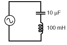
Simple Series Resonance

A similar effect happens in series inductive/capacitive circuits. When a
state of resonance is reached (capacitive and inductive reactances equal),
the two impedances cancel each other out and the total impedance drops to
zero! Example:

	
	Simple series resonant circuit.

Simple series resonant circuit equation
	

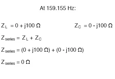With the total series impedance equal to 0 Ω at the resonant frequency of
159.155 Hz, the result is a short circuit across the AC power source at
resonance. In the circuit drawn above, this would not be good.

I’ll add a small resistor (Figure below) in series with the capacitor and
the inductor to keep the maximum circuit current somewhat limited, and
perform another SPICE analysis over the same range of frequencies.
	
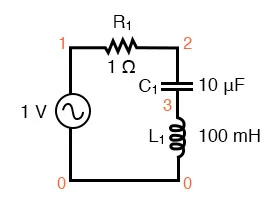	Series resonant circuit suitable for SPICE.

series lc circuit 
 v1 1 0 ac 1 sin 
 r1 1 2 1 
 c1 2 3 10u 
 l1 3 0 100m 
 .ac lin 20 100 200 
 .plot ac i(v1) 
 .end

	
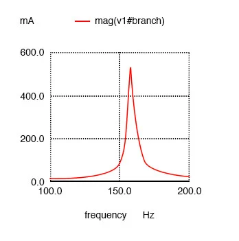	Series resonant circuit plot of current I(v1).

As before, circuit current amplitude increases from bottom to top, while
frequency increases from left to right. The peak is still seen to be at the
plotted frequency point of 157.9 Hz, the closest analyzed point to our
predicted resonance point of 159.155 Hz.

This would suggest that our resonant frequency formula holds as true for
simple series LC circuits as it does for simple parallel LC circuits, which
is the case:
	
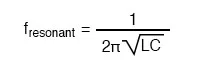	resonant frequency formula

A word of caution is in order with series LC resonant circuits: because of
the high currents which may be present in a series LC circuit at resonance,
it is possible to produce dangerously high voltage drops across the
capacitor and the inductor, as each component possesses significant
impedance.

We can edit the SPICE netlist in the above example to include a plot of
voltage across the capacitor and inductor to demonstrate what happens.

series lc circuit 
 v1 1 0 ac 1 sin 
 r1 1 2 1 
 c1 2 3 10u 
 l1 3 0 100m 
 .ac lin 20 100 200 
 .plot ac i(v1) v(2,3) v(3) 
 .end

	
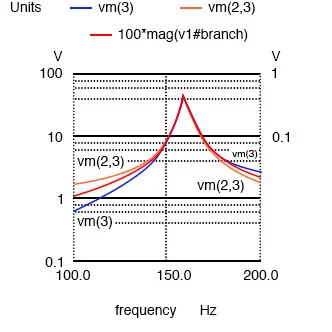	Plot of Vc=V(2,3) 70 V peak, VL=v(3) 70 V peak, I=I(V1#branch) 0.532 A
peak

According to SPICE, the voltage across the capacitor and inductor reaches a
peak somewhere around 70 volts!

This is quite impressive for a power supply that only generates 1 volt.
Needless to say, caution is in order when experimenting with circuits such
as this. The SPICE voltage is lower than the expected value due to the small
(20) number of steps in the AC analysis statement (.ac lin 20 100 200).
What is the expected value?

Given: fr = 159.155 Hz, L = 100mH, R = 1 
 XL = 2πfL = 2π(159.155)(100mH)=j100Ω
 XC = 1/(2πfC) = 1/(2π(159.155)(10µF)) = -j100Ω
 Z = 1 +j100 -j100 = 1 Ω
 I = V/Z = (1 V)/(1 Ω) = 1 A 
 VL = IZ = (1 A)(j100) = j100 V
 VC = IZ = (1 A)(-j100) = -j100 V
 VR = IR = (1 A)(1)= 1 V 
 Vtotal = VL + VC + VR
 Vtotal = j100 -j100 +1 = 1 V
The expected values for capacitor and inductor voltage are 100 V. This voltage
will stress these components to that level and they must be rated accordingly.
However, these voltages are out of phase and cancel, yielding a total voltage
across all three components of only 1 V, the applied voltage.  The ratio of the
capacitor (or inductor) voltage to the applied voltage is the “Q” factor.
Q = VL/VR = VC/VR



REVIEW:

The total impedance of a series LC circuit approaches zero as the power
supply frequency approaches resonance.
The same formula for determining resonant frequency in a simple tank
circuit applies to simple series circuits as well.
Extremely high voltages can be formed across the individual components
of series LC circuits at resonance, due to high current flows and
substantial individual component impedances.






RELATED WORKSHEETS:

    Series and Parallel AC Circuits Worksheet