If the waveform is a pure sine wave, the relationships between amplitudes
(peak-to-peak, peak) and RMS are fixed and known, as they are for any
continuous periodic wave. However, this is not true for an arbitrary
waveform, which may not be periodic or continuous. For a zero-mean sine
wave, the relationship between RMS and peak-to-peak amplitude is:
Peak-to-peak = 2 2 × RMS ≈ 2.8 × RMS . {\displaystyle =2{\sqrt
{2}}\times {\text{RMS}}\approx 2.8\times {\text{RMS}}.}
For other waveforms, the relationships are not the same as they are for
sine
waves. For example, for either a triangular or sawtooth wave
Peak-to-peak = 2 3 × RMS ≈ 3.5 × RMS . {\displaystyle =2{\sqrt
{3}}\times {\text{RMS}}\approx 3.5\times {\text{RMS}}.}
Waveform Variables and operators RMS
DC y = A 0 {\displaystyle y=A_{0}\,} A 0 {\displaystyle A_{0}\,}
Sine wave y = A 1 sin ( 2 π f t ) {\displaystyle y=A_{1}\sin(2\pi
ft)\,} A 1 2 {\displaystyle {\frac {A_{1}}{\sqrt {2}}}}
Square wave y = { A 1 frac ( f t ) < 0.5 − A 1 frac ( f t ) > 0.5 {\displaystyle
y={\begin{cases}A_{1}&\operatorname {frac} (ft)<0.5\\-A_{1}&\operatorname
{frac} (ft)>0.5\end{cases}}} A 1
{\displaystyle A_{1}\,}
DC-shifted square wave y = A 0 + { A 1 frac ( f t ) < 0.5 − A 1 frac ( f t ) > 0.5
{\displaystyle y=A_{0}+{\begin{cases}A_{1}&\operatorname {frac} (ft)
<0.5\\-A_{1}&\operatorname {frac}
(ft)>0.5\end{cases}}} A 0 2 + A 1 2 {\displaystyle {\sqrt
{A_{0}^{2}+A_{1}^{2}}}\,}
Modified sine wave y = { 0 frac ( f t ) < 0.25 A 1 0.25 < frac ( f
t ) < 0.5 0 0.5 < frac ( f t ) < 0.75 − A 1 frac ( f t ) > 0.75
{\displaystyle y={\begin{cases}0&\operatorname {frac} (ft)<
0.25\\A_{1}&0.25<operatorname {frac} (ft)<0.5\\0&0.5<operatorname {frac}
(ft)<0.75\\-A_{1}&\operatorname {frac} (ft)>0.75\end{cases}}} A 1 2
{\displaystyle {\frac {A_{1}}{\sqrt {2}}}}
Triangle wave y = | 2 A 1 frac ( f t ) − A 1 | {\displaystyle
y=\left|2A_{1}\operatorname {frac} (ft)-A_{1}\right|} A 1 3 {\displaystyle
A_{1} \over {\sqrt {3}}}
Sawtooth wave y = 2 A 1 frac ( f t ) − A 1 {\displaystyle
y=2A_{1}\operatorname {frac} (ft)-A_{1}\,} A 1 3 {\displaystyle A_{1}
\over
{\sqrt {3}}}
Pulse wave y = { A 1 frac ( f t ) < D 0 frac ( f t ) > D
{\displaystyle y={\begin{cases}A_{1}&\operatorname {frac} (
ft)<D\\0&\operatorname {frac} (ft)>D\end{cases}}} A 1 D {\displaystyle
A_{1}{\sqrt {D}}}
Phase-to-phase sine wave y = A 1 sin ( t ) − A 1 sin ( t − 2
π
3 ) {\displaystyle y=A_{1}\sin(t)-A_{1}\sin \left(t-{\frac {2\pi
}{3}}\right)\,} A 1 3 2 {\displaystyle A_{1}{\sqrt {\frac {3}{2}}}}
where:
y is displacement,
t is time,
f is frequency,
Ai is amplitude (peak value),
D is the duty cycle or the proportion of the time period (1/f) spent high,
frac(r) is the fractional part of r.
|
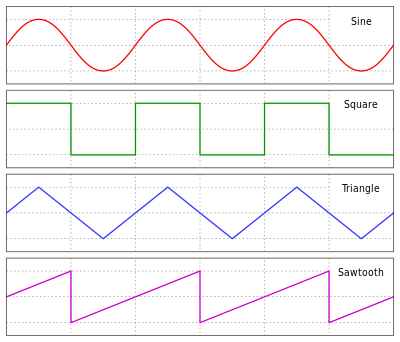 Sine, square, triangle, and sawtooth waveforms. In each, the centerline is
at 0, the positive peak is at y = A 1 {\displaystyle y=A_{1}} and the
negative peak is at y = − A 1 {\displaystyle y=-A_{1}}
Sine, square, triangle, and sawtooth waveforms. In each, the centerline is
at 0, the positive peak is at y = A 1 {\displaystyle y=A_{1}} and the
negative peak is at y = − A 1 {\displaystyle y=-A_{1}}
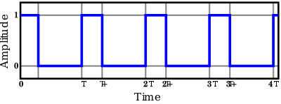 A rectangular pulse wave of duty cycle D, the ratio between the pulse
duration ( τ \tau ) and the period (T); illustrated here with a = 1.
A rectangular pulse wave of duty cycle D, the ratio between the pulse
duration ( τ \tau ) and the period (T); illustrated here with a = 1.
 Graph of a sine wave's voltage vs. time (in degrees), showing RMS, peak
(PK), and peak-to-peak (PP) voltages.
Graph of a sine wave's voltage vs. time (in degrees), showing RMS, peak
(PK), and peak-to-peak (PP) voltages.
|
 Equation 1
This is well understood1 and there is no controversy here.
Now, let’s see how this compares with the value from an rms power calculation.
Figure 1 shows a graph of a 1 V rms sinusoid. The peak-to-peak value is 1 V
rms × 2 √2 = 2.828 V, swinging from +1.414 V to –1.414 V.2
Equation 1
This is well understood1 and there is no controversy here.
Now, let’s see how this compares with the value from an rms power calculation.
Figure 1 shows a graph of a 1 V rms sinusoid. The peak-to-peak value is 1 V
rms × 2 √2 = 2.828 V, swinging from +1.414 V to –1.414 V.2
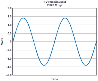 Figure 1. Graph of a 1 V rms sinusoid.
Figure 2 is a graph of the power dissipated by this 1 V rms sinusoid across
a 1 Ω resistor (P = V2/R) that shows:
Figure 1. Graph of a 1 V rms sinusoid.
Figure 2 is a graph of the power dissipated by this 1 V rms sinusoid across
a 1 Ω resistor (P = V2/R) that shows:
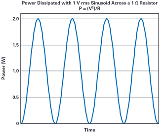 Figure 2. Graph of the power dissipated by a 1 V rms sinusoid across
a 1 Ω resistor.
Figure 2. Graph of the power dissipated by a 1 V rms sinusoid across
a 1 Ω resistor.
 Equation 2
 Equation 3
Author
Doug Ito
Doug Ito is an applications engineer for the High Speed ADC team at Analog
Devices, Inc., San Diego, California. He earned a bachelor’s degree in
electrical engineering from San Diego State University. Doug is a member of
ADI’s EngineerZone® High Speed ADC Support Community.
=======================================================
Equation 3
Author
Doug Ito
Doug Ito is an applications engineer for the High Speed ADC team at Analog
Devices, Inc., San Diego, California. He earned a bachelor’s degree in
electrical engineering from San Diego State University. Doug is a member of
ADI’s EngineerZone® High Speed ADC Support Community.
=======================================================
 x RMS = 1 n ( x 1 2 + x 2 2 + ⋯ + x n 2 ) . {\displaystyle
x_{\text{RMS}}={\sqrt {{\frac {1}{n}}\left({x_{1}}^{2}+{x_{2}}^{2}+\cdots
+{x_{n}}^{2}\right)}}.}
The corresponding formula for a continuous function (or waveform) f(t)
defined over the interval T 1 ≤ t ≤ T 2 T_{1}\leq t\leq T_{2} is
x RMS = 1 n ( x 1 2 + x 2 2 + ⋯ + x n 2 ) . {\displaystyle
x_{\text{RMS}}={\sqrt {{\frac {1}{n}}\left({x_{1}}^{2}+{x_{2}}^{2}+\cdots
+{x_{n}}^{2}\right)}}.}
The corresponding formula for a continuous function (or waveform) f(t)
defined over the interval T 1 ≤ t ≤ T 2 T_{1}\leq t\leq T_{2} is
 f RMS = 1 T 2 − T 1 ∫ T 1 T 2 [ f ( t ) ] 2 d t , {\displaystyle
f_{\text{RMS}}={\sqrt {{1 \over {T_{2}-T_{1}}}{\int
_{T_{1}}^{T_{2}}{[f(t)]}^{2}\,{\rm {d}}t}}},}
and the RMS for a function over all time is
f RMS = 1 T 2 − T 1 ∫ T 1 T 2 [ f ( t ) ] 2 d t , {\displaystyle
f_{\text{RMS}}={\sqrt {{1 \over {T_{2}-T_{1}}}{\int
_{T_{1}}^{T_{2}}{[f(t)]}^{2}\,{\rm {d}}t}}},}
and the RMS for a function over all time is
 f RMS = lim T → ∞ 1 2 T ∫ − T T [ f ( t ) ] 2 d t . {\displaystyle
f_{\text{RMS}}=\lim _{T\rightarrow \infty }{\sqrt {{1 \over {2T}}{\int _{
-T}^{T}{[f(t)]}^{2}\,{\rm {d}}t}}}.}
The RMS over all time of a periodic function is equal to the RMS of one
period
of the function. The RMS value of a continuous function or signal can be
approximated by taking the RMS of a sample consisting of equally spaced
observations. Additionally, the RMS value of various waveforms can also be
determined without calculus, as shown by Cartwright.[4]
In the case of the RMS statistic of a random process, the expected value is
used instead of the mean.
f RMS = lim T → ∞ 1 2 T ∫ − T T [ f ( t ) ] 2 d t . {\displaystyle
f_{\text{RMS}}=\lim _{T\rightarrow \infty }{\sqrt {{1 \over {2T}}{\int _{
-T}^{T}{[f(t)]}^{2}\,{\rm {d}}t}}}.}
The RMS over all time of a periodic function is equal to the RMS of one
period
of the function. The RMS value of a continuous function or signal can be
approximated by taking the RMS of a sample consisting of equally spaced
observations. Additionally, the RMS value of various waveforms can also be
determined without calculus, as shown by Cartwright.[4]
In the case of the RMS statistic of a random process, the expected value is
used instead of the mean.
 RMS Total = RMS 1 2 + RMS 2 2 + ⋯ + RMS n 2 {\displaystyle
{\text{RMS}}_{\text{Total}}={\sqrt {{\text{RMS}}_{1}
^{2}+{\text{RMS}}_{2}^{2}+\cdots +{\text{RMS}}_{n}^{2}}}}
Alternatively, for waveforms that are perfectly positively correlated, or "in
phase"
with each other, their RMS values sum directly.
RMS Total = RMS 1 2 + RMS 2 2 + ⋯ + RMS n 2 {\displaystyle
{\text{RMS}}_{\text{Total}}={\sqrt {{\text{RMS}}_{1}
^{2}+{\text{RMS}}_{2}^{2}+\cdots +{\text{RMS}}_{n}^{2}}}}
Alternatively, for waveforms that are perfectly positively correlated, or "in
phase"
with each other, their RMS values sum directly.
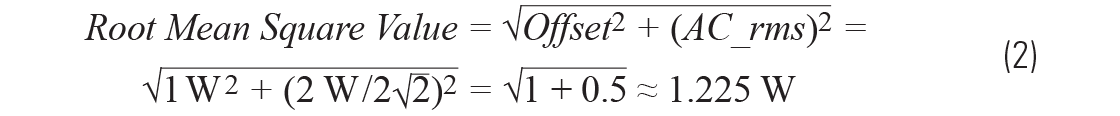
 RMS AC+DC = V DC 2 + RMS AC 2 {\displaystyle {\text
{RMS}}_{\text{AC+DC}}={\sqrt {{\text{V}}_{\text{DC}}
^{2}+{\text{RMS}}_{\text{AC}}^{2}}}}
where V DC {\displaystyle {\text{V}}_{\text{DC}}} refers to the direct
current (or average) component of the signal, and RMS AC {\displaystyle
{\text{RMS}}_{\text{AC}}} is the alternating current component of the
signal.
RMS AC+DC = V DC 2 + RMS AC 2 {\displaystyle {\text
{RMS}}_{\text{AC+DC}}={\sqrt {{\text{V}}_{\text{DC}}
^{2}+{\text{RMS}}_{\text{AC}}^{2}}}}
where V DC {\displaystyle {\text{V}}_{\text{DC}}} refers to the direct
current (or average) component of the signal, and RMS AC {\displaystyle
{\text{RMS}}_{\text{AC}}} is the alternating current component of the
signal.
 P = I 2 R . P=I^{2}R.
However, if the current is a time-varying function, I(t), this formula must
be
extended to reflect the fact that the current (and thus the instantaneous
power)
is varying over time. If the function is periodic (such as household AC
power),
it is still meaningful to discuss the average power dissipated over time,
which
is calculated by taking the average power dissipation:
P = I 2 R . P=I^{2}R.
However, if the current is a time-varying function, I(t), this formula must
be
extended to reflect the fact that the current (and thus the instantaneous
power)
is varying over time. If the function is periodic (such as household AC
power),
it is still meaningful to discuss the average power dissipated over time,
which
is calculated by taking the average power dissipation:
 P a v = ( I ( t ) 2 R ) a v where ( ⋯ ) a v denotes the temporal mean of
a function = ( I ( t ) 2 ) a v R (as R does not vary over time, it can be
factored out) = I RMS 2 R by definition of root-mean-square {\displaystyle
{\begin{aligned}P_{av}&=\left(I(t)^{2}R\right)_{av}&&{\text{where
}}\left(\cdots \right)_{av}{\text{ denotes the temporal mean of a
function}}\\[3pt]&=\left(I(t)^{2}\right)_{av}R&&{\text{(as }}R{\text{ does
not vary over time, it can be factored out)}}\\[3pt]&=I_{\te
xt{RMS}}^{2}R&&{\text{by definition of root-mean-square}}\end{aligned}}}
So, the RMS value, IRMS, of the function I(t) is the constant current that
yields the same power dissipation as the time-averaged power dissipation of
the current I(t).
Average power can also be found using the same method that in the case of a
time-varying voltage, V(t), with RMS value VRMS,
P a v = ( I ( t ) 2 R ) a v where ( ⋯ ) a v denotes the temporal mean of
a function = ( I ( t ) 2 ) a v R (as R does not vary over time, it can be
factored out) = I RMS 2 R by definition of root-mean-square {\displaystyle
{\begin{aligned}P_{av}&=\left(I(t)^{2}R\right)_{av}&&{\text{where
}}\left(\cdots \right)_{av}{\text{ denotes the temporal mean of a
function}}\\[3pt]&=\left(I(t)^{2}\right)_{av}R&&{\text{(as }}R{\text{ does
not vary over time, it can be factored out)}}\\[3pt]&=I_{\te
xt{RMS}}^{2}R&&{\text{by definition of root-mean-square}}\end{aligned}}}
So, the RMS value, IRMS, of the function I(t) is the constant current that
yields the same power dissipation as the time-averaged power dissipation of
the current I(t).
Average power can also be found using the same method that in the case of a
time-varying voltage, V(t), with RMS value VRMS,
 P Avg = V RMS 2 R . {\displaystyle P_{\text{Avg}}={V_{\text{RMS}}^{2}
\over
R}.}
This equation can be used for any periodic waveform, such as a sinusoidal
or
sawtooth waveform, allowing us to calculate the mean power delivered into a
specified load.
By taking the square root of both these equations and multiplying them
together,
the power is found to be:
P Avg = V RMS 2 R . {\displaystyle P_{\text{Avg}}={V_{\text{RMS}}^{2}
\over
R}.}
This equation can be used for any periodic waveform, such as a sinusoidal
or
sawtooth waveform, allowing us to calculate the mean power delivered into a
specified load.
By taking the square root of both these equations and multiplying them
together,
the power is found to be:
 P Avg = V RMS I RMS . {\displaystyle P_{\text{Avg}}
=V_{\text{RMS}}I_{\text{RMS}}.}
Both derivations depend on voltage and current being proportional (that is,
the
load, R, is purely resistive). Reactive loads (that is, loads capable of
not
just dissipating energy but also storing it) are discussed under the topic
of
AC power.
In the common case of alternating current when I(t) is a sinusoidal
current,
as
is approximately true for mains power, the RMS value is easy to calculate
from
the continuous case equation above. If Ip is defined to be the peak
current,
then:
P Avg = V RMS I RMS . {\displaystyle P_{\text{Avg}}
=V_{\text{RMS}}I_{\text{RMS}}.}
Both derivations depend on voltage and current being proportional (that is,
the
load, R, is purely resistive). Reactive loads (that is, loads capable of
not
just dissipating energy but also storing it) are discussed under the topic
of
AC power.
In the common case of alternating current when I(t) is a sinusoidal
current,
as
is approximately true for mains power, the RMS value is easy to calculate
from
the continuous case equation above. If Ip is defined to be the peak
current,
then:
 I RMS = 1 T 2 − T 1 ∫ T 1 T 2 [ I p sin ( ω t ) ] 2 d t ,
{\displaystyle I_{\text{RMS}}={\sqrt {{1 \over {T_{2}-T_{1}}}\int
_{T_{1}}^{T_{2}}\left[I_{\text{p}}\sin(\omega t)\right]^{2}dt}},}
where t is time and ω is the angular frequency (ω = 2π/T, where T is the
period
of the wave).
Since Ip is a positive constant:
I RMS = 1 T 2 − T 1 ∫ T 1 T 2 [ I p sin ( ω t ) ] 2 d t ,
{\displaystyle I_{\text{RMS}}={\sqrt {{1 \over {T_{2}-T_{1}}}\int
_{T_{1}}^{T_{2}}\left[I_{\text{p}}\sin(\omega t)\right]^{2}dt}},}
where t is time and ω is the angular frequency (ω = 2π/T, where T is the
period
of the wave).
Since Ip is a positive constant:
 I RMS = I p 1 T 2 − T 1 ∫ T 1 T 2 sin 2 ( ω t ) d t .
{\displaystyle I_{\text{RMS}}=I_{\text{p}}{\sqrt {{1 \over {T_{2}
-T_{1}}}{\int _{T_{1}}^{T_{2}}{\sin ^{2}(\omega t)}\,dt}}}.}
Using a trigonometric identity to eliminate squaring of trig function:
I RMS = I p 1 T 2 − T 1 ∫ T 1 T 2 sin 2 ( ω t ) d t .
{\displaystyle I_{\text{RMS}}=I_{\text{p}}{\sqrt {{1 \over {T_{2}
-T_{1}}}{\int _{T_{1}}^{T_{2}}{\sin ^{2}(\omega t)}\,dt}}}.}
Using a trigonometric identity to eliminate squaring of trig function:
 I RMS = I p 1 T 2 − T 1 ∫ T 1 T 2 1 − cos ( 2 ω t ) 2 d t = I p
1 T 2 − T 1 [ t 2 − sin ( 2 ω t ) 4 ω ] T 1 T 2 {\displaystyle
{\begin{aligned}I_{\text{RMS}}&=I_{\text{p}}{\sqrt {{1 \over {T_{2}
-T_{1}}}{\int _{T_{1}}^{T_{2}}{1-\cos(2\omega t) \over 2
}\,dt}}}\\[3pt]&=I_{\text{p}}{\sqrt {{1 \over {T_{2}-T_{1}}}\left[{t \over
2}-{\sin(2\omega t) \over 4\omega }\right]_{T_{1}}^{T_{2}}}}\end{aligned}}}
but since the interval is a whole number of complete cycles (per definition
of RMS), the sine terms will cancel out, leaving:
I RMS = I p 1 T 2 − T 1 ∫ T 1 T 2 1 − cos ( 2 ω t ) 2 d t = I p
1 T 2 − T 1 [ t 2 − sin ( 2 ω t ) 4 ω ] T 1 T 2 {\displaystyle
{\begin{aligned}I_{\text{RMS}}&=I_{\text{p}}{\sqrt {{1 \over {T_{2}
-T_{1}}}{\int _{T_{1}}^{T_{2}}{1-\cos(2\omega t) \over 2
}\,dt}}}\\[3pt]&=I_{\text{p}}{\sqrt {{1 \over {T_{2}-T_{1}}}\left[{t \over
2}-{\sin(2\omega t) \over 4\omega }\right]_{T_{1}}^{T_{2}}}}\end{aligned}}}
but since the interval is a whole number of complete cycles (per definition
of RMS), the sine terms will cancel out, leaving:
 I RMS = I p 1 T 2 − T 1 [ t 2 ] T 1 T 2 = I p 1 T 2 − T 1 T 2 − T 1
2
= I p2
. {\displaystyle I_{\text{RMS}}=I_{\text{p}}{\sqrt {{1 \over {T_{2}
-T_{1}}}\left[{t \over 2}\right]_{T_{1}}^{T_{2}}}}=I_{\text{p}}{\sqrt {{1
\over {T_{2}-T_{1}}}{{T_{2}-T_{1}} \over 2}}}={I_{\text{p}} \over {\sqrt
{2}}}.}
A similar analysis leads to the analogous equation for sinusoidal voltage:
I RMS = I p 1 T 2 − T 1 [ t 2 ] T 1 T 2 = I p 1 T 2 − T 1 T 2 − T 1
2
= I p2
. {\displaystyle I_{\text{RMS}}=I_{\text{p}}{\sqrt {{1 \over {T_{2}
-T_{1}}}\left[{t \over 2}\right]_{T_{1}}^{T_{2}}}}=I_{\text{p}}{\sqrt {{1
\over {T_{2}-T_{1}}}{{T_{2}-T_{1}} \over 2}}}={I_{\text{p}} \over {\sqrt
{2}}}.}
A similar analysis leads to the analogous equation for sinusoidal voltage:
 V RMS = V p 2 , {\displaystyle V_{\text{RMS}}={V_{\text{p}} \over {\sqrt
{2}}},}
where IP represents the peak current and VP represents the peak voltage.
Because of their usefulness in carrying out power calculations, listed
voltages for power outlets (for example, 120 V in the US, or 230 V in
Europe) are almost always quoted in RMS values, and not peak values. Peak
values can be calculated from RMS values from the above formula, which
implies VP = VRMS × √2, assuming the source is a pure sine wave. Thus
the
peak value of the mains voltage in the USA is about 120 × √2, or about
170 volts. The peak-to-peak voltage, being double this, is about 340 volts.
A similar calculation indicates that the peak mains voltage in Europe is
about 325 volts, and the peak-to-peak mains voltage, about 650 volts.
RMS quantities such as electric current are usually calculated over one
cycle. However, for some purposes the RMS current over a longer period is
required when calculating transmission power losses. The same principle
applies, and (for example) a current of 10 amps used for 12 hours each 24
-hour day represents an average current of 5 amps, but an RMS current of
7.07 amps, in the long term.
The term RMS power is sometimes erroneously used in the audio industry as a
synonym for mean power or average power (it is proportional to the square
of
the RMS voltage or RMS current in a resistive load). For a discussion of
audio power measurements and their shortcomings, see Audio power.
V RMS = V p 2 , {\displaystyle V_{\text{RMS}}={V_{\text{p}} \over {\sqrt
{2}}},}
where IP represents the peak current and VP represents the peak voltage.
Because of their usefulness in carrying out power calculations, listed
voltages for power outlets (for example, 120 V in the US, or 230 V in
Europe) are almost always quoted in RMS values, and not peak values. Peak
values can be calculated from RMS values from the above formula, which
implies VP = VRMS × √2, assuming the source is a pure sine wave. Thus
the
peak value of the mains voltage in the USA is about 120 × √2, or about
170 volts. The peak-to-peak voltage, being double this, is about 340 volts.
A similar calculation indicates that the peak mains voltage in Europe is
about 325 volts, and the peak-to-peak mains voltage, about 650 volts.
RMS quantities such as electric current are usually calculated over one
cycle. However, for some purposes the RMS current over a longer period is
required when calculating transmission power losses. The same principle
applies, and (for example) a current of 10 amps used for 12 hours each 24
-hour day represents an average current of 5 amps, but an RMS current of
7.07 amps, in the long term.
The term RMS power is sometimes erroneously used in the audio industry as a
synonym for mean power or average power (it is proportional to the square
of
the RMS voltage or RMS current in a resistive load). For a discussion of
audio power measurements and their shortcomings, see Audio power.
 v RMS = 3 R T M {\displaystyle v_{\text{RMS}}={\sqrt {3RT \over M}}}
where R represents the gas constant, 8.314 J/(mol·K), T is the temperature
of the gas in kelvins, and M is the molar mass of the gas in kilograms per
mole. In physics, speed is defined as the scalar magnitude of velocity. For
a stationary gas, the average speed of its molecules can be in the order of
thousands of km/h, even though the average velocity of its molecules is
zero.
v RMS = 3 R T M {\displaystyle v_{\text{RMS}}={\sqrt {3RT \over M}}}
where R represents the gas constant, 8.314 J/(mol·K), T is the temperature
of the gas in kelvins, and M is the molar mass of the gas in kilograms per
mole. In physics, speed is defined as the scalar magnitude of velocity. For
a stationary gas, the average speed of its molecules can be in the order of
thousands of km/h, even though the average velocity of its molecules is
zero.
 ∑ n = 1 N x 2 [ n ] = 1 N ∑ m = 1 N | X [ m ] | 2 , {\displaystyle
\sum
_{n=1}^{N}{x^{2}[n]}={\frac {1}{N}}\sum _{m=1}^{N}\left|X[m]\right|^{2},}
where X [ m ] = FFT { x [ n ] } {\displaystyle X[m]=\operatorname {FFT}
\{x[n]\}} and N is the sample size, that is, the number of observations in
the sample and FFT coefficients.
In this case, the RMS computed in the time domain is the same as in the
frequency domain:
∑ n = 1 N x 2 [ n ] = 1 N ∑ m = 1 N | X [ m ] | 2 , {\displaystyle
\sum
_{n=1}^{N}{x^{2}[n]}={\frac {1}{N}}\sum _{m=1}^{N}\left|X[m]\right|^{2},}
where X [ m ] = FFT { x [ n ] } {\displaystyle X[m]=\operatorname {FFT}
\{x[n]\}} and N is the sample size, that is, the number of observations in
the sample and FFT coefficients.
In this case, the RMS computed in the time domain is the same as in the
frequency domain:
 RMS { x [ n ] } = 1 N ∑ n x 2 [ n ] = 1 N 2 ∑ m | X [ m ] | 2 = ∑ m
|
X [ m ] N | 2 . {\displaystyle {\text{RMS}}\{x[n]\}={\sqrt {{\frac
{1}{N}}\sum _{n}{x^{2}[n]}}}={\sqrt {{\frac {1}{N^{2}}}\sum _{m}{{\bigl
|}X[m]{\bigr |}}^{2}}}={\sqrt {\sum _{m}{\left|{\frac
{X[m]}{N}}\right|^{2}}}}.}
RMS { x [ n ] } = 1 N ∑ n x 2 [ n ] = 1 N 2 ∑ m | X [ m ] | 2 = ∑ m
|
X [ m ] N | 2 . {\displaystyle {\text{RMS}}\{x[n]\}={\sqrt {{\frac
{1}{N}}\sum _{n}{x^{2}[n]}}}={\sqrt {{\frac {1}{N^{2}}}\sum _{m}{{\bigl
|}X[m]{\bigr |}}^{2}}}={\sqrt {\sum _{m}{\left|{\frac
{X[m]}{N}}\right|^{2}}}}.}
 x rms 2 = x ¯ 2 + σ x 2 = x 2 ¯ . {\displaystyle
x_{\text{rms}}^{2}={\overline {x}}^{2}+\sigma _{x}^{2}={\overline
{x^{2}}}.}
From this it is clear that the RMS value is always greater than or equal to
the
average, in that the RMS includes the "error" / square deviation as well.
Physical scientists often use the term root mean square as a synonym for
standard deviation when it can be assumed the input signal has zero mean,
that
is, referring to the square root of the mean squared deviation of a signal
from
a given baseline or fit.[8][9] This is useful for electrical engineers in
calculating the "AC only" RMS of a signal. Standard deviation being the RMS of
a signal's variation about the mean, rather than about 0, the DC component
is
removed (that is, RMS(signal) = stdev(signal) if the mean signal is 0).
x rms 2 = x ¯ 2 + σ x 2 = x 2 ¯ . {\displaystyle
x_{\text{rms}}^{2}={\overline {x}}^{2}+\sigma _{x}^{2}={\overline
{x^{2}}}.}
From this it is clear that the RMS value is always greater than or equal to
the
average, in that the RMS includes the "error" / square deviation as well.
Physical scientists often use the term root mean square as a synonym for
standard deviation when it can be assumed the input signal has zero mean,
that
is, referring to the square root of the mean squared deviation of a signal
from
a given baseline or fit.[8][9] This is useful for electrical engineers in
calculating the "AC only" RMS of a signal. Standard deviation being the RMS of
a signal's variation about the mean, rather than about 0, the DC component
is
removed (that is, RMS(signal) = stdev(signal) if the mean signal is 0).
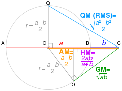 Geometric proof without words that max (a,b) > root mean square (RMS) or
quadratic mean (QM) > arithmetic mean (AM) > geometric mean (GM) > harmonic
mean (HM) > min (a,b) of two distinct positive numbers a and b [note 1]
Geometric proof without words that max (a,b) > root mean square (RMS) or
quadratic mean (QM) > arithmetic mean (AM) > geometric mean (GM) > harmonic
mean (HM) > min (a,b) of two distinct positive numbers a and b [note 1]