Abstract gprMax is open source software that simulates electromagnetic wave propagation, using the Finite-Difference Time-Domain (FDTD) method, for the numerical modelling of Ground Penetrating Radar (GPR). gprMax was originally developed in 1996 when numerical modelling using the FDTD method and, in general, the numerical modelling of GPR were in their infancy. Current computing resources offer the opportunity to build detailed and complex FDTD models of GPR to an extent that was not previously possible. To enable these types of simulations to be more easily realised, and also to facilitate the addition of more advanced features, gprMax has been redeveloped and significantly modernised. The original C-based code has been completely rewritten using a combination of Python and Cython programming languages. Standard and robust file formats have been chosen for geometry and field output files. New advanced modelling features have been added including: an unsplit implementation of higher order Perfectly Matched Layers (PMLs) using a recursive integration approach; diagonally anisotropic materials; dispersive media using multi-pole Debye, Drude or Lorenz expressions; soil modelling using a semi-empirical formulation for dielectric properties and fractals for geometric characteristics; rough surface generation; and the ability to embed complex transducers and targets.
Program summary Program title: gprMax Catalogue identifier: AFBG_v1_0 Program summary URL:http://cpc.cs.qub.ac.uk/summaries/AFBG_v1_0.html Program obtainable from: CPC Program Library, Queen’s University, Belfast, N. Ireland Licensing provisions: GNU GPL v3 No. of lines in distributed program, including test data, etc.: 627180 No. of bytes in distributed program, including test data, etc.: 26762280 Distribution format: tar.gz Programming language: Python. Computer: Any computer with a Python interpreter and a C compiler. Operating system: Microsoft Windows, Mac OS X, and Linux. RAM: Problem dependent Classification: 10. External routines: Cython[1], h5py[2], matplotlib[3], NumPy[4], mpi4py[5] Nature of problem: Classical electrodynamics Solution method: Finite-Difference Time-Domain (FDTD) Running time: Problem dependent References: [1] Cython, http://www.cython.org [2] h5py, http://www.h5py.org [3] matplotlib, http://www.matplotlib.org [4] NumPy, http://www.numpy.org [5] mpi4py, http://mpi4py.scipy.org Previous article in issue Next article in issue
Keywords Computational electromagnetism Ground Penetrating Radar Finite-Difference Time-Domain Open source Python
1. Introduction Ground Penetrating Radar (GPR) is a powerful non-destructive tool that is used for many diverse applications in fields such as engineering, geophysics and even medicine. Examples include: infrastructure assessment of bridges, roads, and railways; locating buried utilities; ice profiling and glaciology; groundwater and soil contaminant mapping; landmine and unexploded ordnance (UXO) recognition; and detection of breast cancer tumours. Understanding how electromagnetic waves propagate through naturally occurring or man-made heterogeneous environments is a challenging problem. Consequently the interpretation of data acquired using GPR is often difficult due to the complex interactions between the GPR system, the target(s) of interest, and the environment. This is especially evident when trying to interpret quantitative information from GPR data. Successful interpretation of GPR data usually relies on considerable experience gained through extensive experimentation, and even then is often limited to identifying areas of interest or anomalies in the data. To advance our understanding of GPR as well as provide a means for testing new data processing techniques and interpretation algorithms it is important to have accurate and robust simulation software. gprMax is open source software that simulates electromagnetic wave propagation for the numerical modelling of GPR, and is available from http://www.gprmax.com . It uses Yee’s [1] algorithm (with second order accurate derivatives in space and time) to solve Maxwell’s equations in 3D using the Finite -Difference Time-Domain (FDTD) method. The FDTD method is a differential -equation-based solver that has been described in many publications, such as [2], so will not be repeated here. In summary, the strengths of the FDTD method are that it is a simple, fully explicit, general, and robust technique. The main weakness is due to the fact that the entire computational domain must be discretised which can require extensive computational resources. The time-domain nature of the FDTD method means in a single simulation a wide range of frequencies can be modelled. This is particularly well-suited for simulating GPR systems which are usually ultra wide-band (UWB). However, the computational domain must still be discretised in relation to the highest frequency of interest. gprMax was originally developed in 1996 [3] when numerical modelling using the FDTD method and, in general, the numerical modelling of GPR were in their infancy. Since then a number of commercial [4], [5] and other freely -available [6], [7] FDTD-based solvers have become available, but gprMax has remained one of the most widely used simulation tools in the GPR community. It has been successfully used for a diverse range of applications in academia and industry [8], [9], [10], [11], [12], [13], and has been cited more than 200 times since 2005 [14]. Computing power has increased dramatically since gprMax was initially developed—multi-core CPUs and gigabytes of RAM are now standard features on desktop and laptop machines, and many research institutions now have their own high-performance computing (HPC) systems. These computational advances have particularly benefited numerical techniques, such as FDTD, that discretise the entire computational domain, and thus larger and more complex scenarios can be investigated. To enable these types of problems to be simulated using gprMax, we have made significant modernisations to the code and also added of new advanced features to the software. The paper is organised as follows: Section 2 provides an overview of the design of the software, the tools that were used, and the principles behind some of the design choices; Section 3 describes the key advanced features that have been developed for modelling GPR; and finally Section 4 gives examples of GPR simulations that take advantage of many of these new features.
2. Software overview
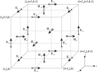
2.1. Design principles and general features gprMax was developed as cross-platform software for Linux, Microsoft Windows, and later Mac OS X. It was originally written using the C programming language, with the computationally intensive parts–the FDTD solver loops–parallelised using OpenMP [15]. The original design principal was to create a general computational electromagnetic solver, and then build features specifically for modelling GPR onto that core. We continued to use this philosophy for the redesign of gprMax whilst also considering how to facilitate the implementation of new advanced features, and how to lay better foundations for future developments. We decided that the code should be rewritten in Python [16]—a modern, interpreted language that is intended to be highly readable and extensible. There are advantageous features of Python such as dynamic typing, automatic memory management, and object orientation. However some of these attributes come at a performance cost compared with statically typed languages such as C. For a typical FDTD solver, most of the computational time is spent solving the electromagnetic field update equations. Therefore we focused object orientation and abstraction on the parts of the code that construct the model (prior to the solving), and then used Cython [17]–a superset of Python that generates efficient C source code that can be compiled into extension modules–to write simple methods with minimal decision-making for the FDTD solver. Additionally, Cython supports OpenMP which allowed the FDTD solver to be multi-threaded on machines with multiple CPUs/cores. As an example of this design philosophy, materials have their own class and methods but prior to the solving phase, the update coefficients for the electric and magnetic field equations for each material are stored in simple floating-point NumPy arrays. A NumPy array of integers is used to represent materials and their locations in the computational domain, i.e. the geometry of the model. The integers provide a lookup (index) into the array of the actual material properties/coefficients. Therefore a significant memory saving is made by not having to store material properties/coefficients at every location in the computational domain. We used MPI for Python (mpi4py) [18] to implement a simple MPI task farm to distribute series of models as independent tasks. This is especially useful in many GPR simulations where a B-scan1 is required. Each A-scan2 can be task-farmed as an independent model. The option to combine OpenMP for threading within an individual model and use MPI to distribute a series of models, can be extremely beneficial in HPC environments. gprMax originally consisted of two simulators—GprMax2D, which solved the transverse-magnetic mode with respect to the z-direction (TMz) in 2D, and GprMax3D which solved the full FDTD algorithm in 3D. Although there were a lot of similarities between the two simulators, two separate codebases had to be maintained which was not efficient. Ever increasing computational power has meant 3D simulations are more accessible and common, but despite this there is still often a need to run simple 2D simulations, especially for educational purposes. Therefore we designed a single codebase that can run 2D or 3D simulations. A 2D simulation is achieved by specifying a computational domain that has only a single cell dimension in one direction (that direction is considered the infinite direction). For example, referring to Fig. 1 which shows a 3D Yee cell, if we assume that the infinite direction is the z-direction, the software will set the values of the electric field components on the z-faces of the cell to zero, i.e. the and components. This has the effect of setting the component to zero and therefore making Perfect Electric Conductor (PEC) boundaries in the z -direction. The field components that remain are , , and , giving a 2D TMz mode. It is possible to relax the time step from the (default) equality with the Courant Friedrichs Lewy (CFL) condition in 3D to the 2D equivalent.
 Download : Download high-res image (174KB)
Download : Download full-size image
Fig. 1. FDTD Yee cell.
2.2. User interface, scripting and file formats
gprMax uses a text-based input file in which users specify all of the
parameters for a simulation, e.g., model size, discretisation, time window,
geometry, materials, and excitation, via pre-defined commands. We considered
developing a CAD-based graphical user interface (GUI) or creating a pure
programming interface for gprMax but decided against both of these options.
There were three guiding principles behind this design decision (two are
similar to those given in [7]): firstly, users most often perform a series
of related simulations with varying parameters to solve or optimise a
particular problem; secondly, we wanted users to be able to easily create
models with minimal knowledge or experience of programming; and thirdly we
decided the limited resources we had were best concentrated on developing
advanced modelling features for GPR within software that could easily
interface with other tools. Although a CAD-based GUI is useful for creating
single simulations it becomes increasingly cumbersome for a series of
simulations or where simulations contain heterogeneities, e.g. a model of a
soil with stochastically varying electrical properties.
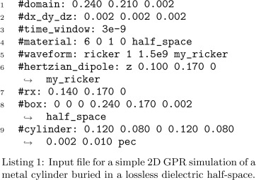
Listing 1 provides an example of an input file for a simple 2D GPR
simulation of a metal cylinder buried in a lossless dielectric half-space.
Fig. 2 shows the geometry of the model.
Download : Download high-res image (174KB)
Download : Download full-size image
Fig. 1. FDTD Yee cell.
2.2. User interface, scripting and file formats
gprMax uses a text-based input file in which users specify all of the
parameters for a simulation, e.g., model size, discretisation, time window,
geometry, materials, and excitation, via pre-defined commands. We considered
developing a CAD-based graphical user interface (GUI) or creating a pure
programming interface for gprMax but decided against both of these options.
There were three guiding principles behind this design decision (two are
similar to those given in [7]): firstly, users most often perform a series
of related simulations with varying parameters to solve or optimise a
particular problem; secondly, we wanted users to be able to easily create
models with minimal knowledge or experience of programming; and thirdly we
decided the limited resources we had were best concentrated on developing
advanced modelling features for GPR within software that could easily
interface with other tools. Although a CAD-based GUI is useful for creating
single simulations it becomes increasingly cumbersome for a series of
simulations or where simulations contain heterogeneities, e.g. a model of a
soil with stochastically varying electrical properties.
Listing 1 provides an example of an input file for a simple 2D GPR
simulation of a metal cylinder buried in a lossless dielectric half-space.
Fig. 2 shows the geometry of the model.
 Download : Download high-res image (141KB)
Download : Download full-size image
Fig. 2. FDTD mesh of metal cylinder buried in a lossless dielectric half
-space.
Download : Download high-res image (141KB)
Download : Download full-size image
Fig. 2. FDTD mesh of metal cylinder buried in a lossless dielectric half
-space.
 Download : Download high-res image (304KB)
Download : Download full-size image
All commands begin with a hash symbol followed by the name of the command,
and then a list of associated parameters.3 In lines 1–2 the size of the
computational domain and discretisation of the model are given in x, y, z
directions. The model is 2D as the z dimension of the domain is only a
single cell. Line 3 specifies the duration of time to simulate, with the
time step being calculated automatically at the CFL limit. In line 4 a
material is defined which is used to build the half-space. The material has
the identifier name half_space, a relative permittivity of six, electric
conductivity of zero (S/m), relative permeability of one, and zero magnetic
loss (
). A Hertzian dipole fed with a Ricker waveform with a centre frequency of
1.5 GHz is used as a source (lines 5–6). A receiver is used to record the
time histories of the electric and magnetic fields at a specific location
for the duration of the simulation. Finally, a box object (used to represent
the half-space) and a cylinder object are created. The identifiers
half_space and pec4 refer to the materials that the objects are built from.
The order of the objects is important as a layered canvas approach is used,
i.e. subsequent objects overwrite the properties of previous objects if they
specify the same location. The full syntax of every command can be found in
the User Guide (http://docs.gprmax.com
).
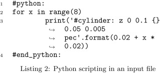
We have made it easier to create more complex simulations in gprMax by
allowing scripting in the input file. This is achieved because blocks of
Python code can be written in the input file and are then executed when the
file is read. Listing 2 shows a simple example of how a repetitive geometry
command can be scripted directly in the input file using a for loop in
Python. A PEC cylinder extending from 0 to 100 mm in the z-direction, with y
-coordinate 50 mm, and radius 5 mm, is repeated every 20 mm in the x
-direction from 20 mm to 160 mm.
Download : Download high-res image (304KB)
Download : Download full-size image
All commands begin with a hash symbol followed by the name of the command,
and then a list of associated parameters.3 In lines 1–2 the size of the
computational domain and discretisation of the model are given in x, y, z
directions. The model is 2D as the z dimension of the domain is only a
single cell. Line 3 specifies the duration of time to simulate, with the
time step being calculated automatically at the CFL limit. In line 4 a
material is defined which is used to build the half-space. The material has
the identifier name half_space, a relative permittivity of six, electric
conductivity of zero (S/m), relative permeability of one, and zero magnetic
loss (
). A Hertzian dipole fed with a Ricker waveform with a centre frequency of
1.5 GHz is used as a source (lines 5–6). A receiver is used to record the
time histories of the electric and magnetic fields at a specific location
for the duration of the simulation. Finally, a box object (used to represent
the half-space) and a cylinder object are created. The identifiers
half_space and pec4 refer to the materials that the objects are built from.
The order of the objects is important as a layered canvas approach is used,
i.e. subsequent objects overwrite the properties of previous objects if they
specify the same location. The full syntax of every command can be found in
the User Guide (http://docs.gprmax.com
).
We have made it easier to create more complex simulations in gprMax by
allowing scripting in the input file. This is achieved because blocks of
Python code can be written in the input file and are then executed when the
file is read. Listing 2 shows a simple example of how a repetitive geometry
command can be scripted directly in the input file using a for loop in
Python. A PEC cylinder extending from 0 to 100 mm in the z-direction, with y
-coordinate 50 mm, and radius 5 mm, is repeated every 20 mm in the x
-direction from 20 mm to 160 mm.
 Download : Download high-res image (129KB)
Download : Download full-size image
Alongside improvements to the input file we have introduced new file formats
for field outputs and geometry information. We wanted to design gprMax to be
as flexible as possible and based around robust and standardised formats
which would allow users a choice of tools for creating input, and viewing
and processing output. We have used HDF5 [19] as the output file format to
handle the larger and more complex data sets that are being generated. HDF5
is a robust, portable and extensible format with a number of free readers
available. The Visualization Toolkit (VTK) [20] is used for improved
handling and viewing of the FDTD geometry meshes. The VTK is an open source
system for 3D computer graphics, image processing and visualisation. It also
has a number of free readers available such as Paraview
(http://www.paraview.org
). gprMax allows the user to view geometry information for the entire model
domain or any specified sub-volume within the model domain. The geometry
information can be requested on a per-cell basis, useful for viewing
volumetric objects, or a per-cell-edge basis, which is useful for viewing
fine or more complex geometrical features.
3. Advanced features for modelling GPR
gprMax contains many powerful and customisable features for modelling GPR.
This section focuses on a selection of the new and advanced capabilities
that have been developed.
3.1. Library of antenna models
Models of antennas have been included in numerical simulations of GPR
intermittently over the past 20 years with varying degrees of realism. Those
that have included models of the actual antenna have been mainly of antennas
used in academia or for research purposes [21], [22], [23], [24], [25],
[26], [27], [28], [29], [30]. There has been very limited published work of
GPR simulations with models of commercial antennas [31], [32], [33], [34].
In fact, many simulations have used a theoretical Hertzian dipole source to
represent a real GPR antenna where only far-field behaviour or travel-time
information was of interest, or where computational resources were limited.
However, advances in computational power, coupled with the desire to
investigate quantitative amplitude information from GPR, means there is a
need to develop and use detailed 3D FDTD models of realistic GPR antennas in
simulations.
gprMax now includes a library with pre-defined models of antennas that
behave similarly to commercial antennas. Currently, models of antennas
similar to Geophysical Survey Systems, Inc. (GSSI) (
http://www.geophysical.com
) 1.5 GHz (Model 5100) antenna, and MALA Geoscience (http://www.malags.com/
) 1.2 GHz antenna are included. This simplifies the process of adding such
intricate structures into a model. Listing 3 demonstrates how a model of a
high-frequency GPR antenna, shown in Fig. 3, can be inserted into a
simulation without having to be built step-by-step by the user. The antenna
model is imported from a library and inserted at a specific location in the
computational domain.
Download : Download high-res image (933KB)
Download : Download full-size image
Fig. 3. A model of a high-frequency antenna like a MALA 1.2 GHz antenna. The
geometry mesh is a combination of per-cell geometry information for
volumetric objects, and per-cell-edge geometry information for finer
geometric details.
Download : Download high-res image (153KB)
Download : Download full-size image
3.2. Absorbing boundary conditions
With increased research into quantitative amplitude information from GPR, it
has become necessary for simulations to have more efficient and better
-performing Perfectly Matched Layer (PML) absorbing boundary conditions
(ABC). Since 2005 gprMax has featured PML ABCs based on the uniaxial PML
(UPML) [35]formulation. A PML based on a recursive integration (RI)
approach to the complex frequency shifted (CFS) PML [36] has now been
developed for gprMax. The implementation is such that a standard UPML, first
order CFS-PML, or second order mixed RIPML can now be configured.
Additionally, for advanced usage, the parameters of the PML can be
customised, which allows the performance of the PML to be better optimised
for specific applications. One of the attractions of the RIPML is that it is
easily applied as a correction to the electric and magnetic field values
after the complete FDTD grid has been updated using the standard FDTD update
equations. Moreover, the RIPML is media agnostic so it can be used, without
change, to problems involving dispersive and anisotropic materials.
3.3. Materials
Many of the environments where GPR is used are complex, heterogeneous, and
contain materials with dispersive properties. Therefore we have focused on
developing new features and making improvements to how materials are created
and simulated in the software.
3.3.1. Anisotropic materials
gprMax allows anisotropic objects to be modelled in a simulation. Materials
such as wood and fibre-reinforced composites, which are often imaged with
GPR, can now be more accurately described. This has been achieved by
enabling every volumetric geometry object to specify up to three material
identifiers. It is therefore possible for every object to have diagonal
anisotropy. Listing 4 demonstrates the uniaxial anisotropy of a carbon-fibre
-reinforced polymer (CFRP) composite material.
Download : Download high-res image (163KB)
Download : Download full-size image
The material cfrpX is used to define the material properties of the CFRP in
the x direction, and the material cfrpYZ for the y and z directions. A box
of CFRP is created on line 3, with the object using three identifiers to
associate it with its materials properties in the x, y, z directions.
3.3.2. Dispersive materials
gprMax has always included the ability to represent dispersive materials
using a single-pole Debye model. Many materials can be adequately
represented using this approach for the typical frequency ranges associated
with GPR. However, multi-pole Debye, Drude and Lorenz functions are often
used to simulate the electric susceptibility of materials such as: water
[37], human tissue [38], cold plasma [39], gold [40], and soils [41],
[42], [29]. Electric susceptibility relates the polarisation density to the
electric field, and includes both the real and imaginary parts of the
complex electric permittivity variation. gprMax now uses a recursive
convolution based method to express dispersive properties as apparent
current density sources [43]. A major advantage of this implementation is
that it creates an inclusive susceptibility function that holds, as special
cases, Debye, Drude and Lorenz materials. Listing 5 gives an example of the
command to add a 2-pole Debye material that simulates human fatty tissue
[38].
Download : Download high-res image (146KB)
Download : Download full-size image
Line 1 defines the basic material properties5 and in line 2 the
#add_dispersion_debye command adds dispersive behaviour to the material
based on the Debye formulation. The parameters for the #add_dispersion_debye
command define the number of poles, the difference between the DC (static)
relative permittivity and the relative permittivity at infinite frequency
for the first Debye pole, the relaxation time (seconds) for the first Debye
pole, the difference between the DC (static) relative permittivity and the
relative permittivity at infinite frequency for the second Debye pole, and
the relaxation time (seconds) for the second Debye pole.
3.3.3. Soil models and topography
The inclusion of improved models of soils is important for many GPR
simulations. gprMax can now be used to create soils with more realistic
dielectric and geometrical properties [44]. A semi-empirical model,
initially suggested by [45], is used to describe the dielectric properties
of the soil. The model relates relative the permittivity of the soil to its
bulk density, sand particle density, sand fraction, clay fraction and
volumetric water fraction. Using this approach, a more realistic soil with a
stochastic distribution of the aforementioned parameters can be modelled.
The real and imaginary parts of this semi-empirical model can be
approximated using a multi-pole Debye function plus a conductive term. This
can now be achieved in gprMax using the new dispersive material
functionality described in Section 3.3.2. For example, to create a soil
with bulk density,
, sand particle density, , sand fraction, , clay fraction,
, and a volumetric water fraction in the range 0.001–0.25, the command
#soil_peplinski: 0.5 0.5 2 2.66 0.001 0.25 soil_properties would be used.
Fractals are scale invariant functions and can be used to express the
topography of soils for a wide range of scales with sufficient detail [46].
Fractals can be generated by the convolution of Gaussian noise with the
inverse Fourier transform of
, where is the wavenumber and
is a constant related to the fractal dimension [47].
The combination of the Peplinski soil models and the fractal functions can
be used to generate a soil model in gprMax with more realistic dielectric
and geometrical properties. Listing 6 gives an example of the commands
required to generate the soil model shown in Fig. 4. The soil is composed of
ten different dispersive materials and features a rough surface.
Download : Download high-res image (444KB)
Download : Download full-size image
Fig. 4. Stochastic distribution of an arbitrarily chosen property of the
soil and a rough surface created using fractal correlated noise.
Download : Download high-res image (192KB)
Download : Download full-size image
4. Example GPR simulations
The following three examples demonstrate how simple and more advanced
simulations of GPR that can be carried out using gprMax.
4.1. B-scan of a buried cylindrical object
This is an example of a B-scan from a simple 2D GPR simulation of a metal
cylinder buried in a lossless dielectric half-space. Listing 7 is the input
file required to generate this model.
Download : Download high-res image (292KB)
Download : Download full-size image
Listing 7 is identical to Listing 1 except that to create the B-scan the
source and receiver are moved in steps to a new position every time the
simulation is run, i.e. for each A-scan. The resulting B-scan is shown in
Fig. 5 and is composed of 60 A-scans, i.e. 60 model runs.
Download : Download high-res image (260KB)
Download : Download full-size image
Fig. 5. B-scan of a metal cylinder buried in a homogeneous dielectric half
-space.
4.2. Antenna patterns in a heterogeneous soil
This example shows how to simulate the field patterns of a GPR antenna over
a heterogeneous soil.
Download : Download high-res image (791KB)
Download : Download full-size image
Listing 8 demonstrates using Python scripting within an input file to
generate the model. Fig. 6 shows a series of the resulting
-plane field patterns at different observation distances from the antenna.
Further research into the characteristics of GPR antennas in lossless and
lossy environments can be found in [31], [34], [48].
Download : Download high-res image (703KB)
Download : Download full-size image
Fig. 6.
-plane field pattern from GSSI 1.5 GHz antenna model over a lossy,
heterogeneous soil.
4.3. Complex environment
The geometry of the final example model is shown in Fig. 7. The simulation
is of a complex environment that can be often be encountered in GPR surveys.
It includes a heterogeneous soil with a rough surface and pools of surface
water. Grass and roots are simulated, and a model of GPR antenna is
included. Listing 9 shows that all of this complexity is achieved using
relatively few commands which demonstrates the power and ease of use of the
software.
Download : Download high-res image (402KB)
Download : Download full-size image
Fig. 7. Model of a GPR in a complex environment.
Download : Download high-res image (408KB)
Download : Download full-size image
5. Conclusion
Current computing resources offer the possibility to build ever larger and
more complex simulations of GPR that have not been possible before. A new
version of gprMax has been developed that is open source and written using
Python and Cython programming languages. Improvements have been made to
existing features of gprMax as well as the addition of new advanced
modelling features including: an unsplit implementation of higher order
perfectly matched layers (PMLs) using a recursive integration approach;
diagonally anisotropic materials; dispersive media using multi-pole Debye,
Drude or Lorenz expressions; soil modelling using a semi-empirical
formulation for dielectric properties and fractals for geometric
characteristics; rough surface generation; and the ability to embed complex
transducers and targets. A series of example simulations demonstrate some of
these features and the ease with which they can be used. The open source
principle of the software provides a platform for developers to contribute
new ideas and algorithms which will be of future benefit to the GPR research
community.
Acknowledgements
This work was supported by The Defence Science and Technology Laboratory
(Dstl), UK, and the Engineering and Physical Sciences Research Council
(EPSRC), UK (grant no. EP/J501943/1), and benefited from networking
activities carried out within the EU funded COST Action TU1208 “Civil
Engineering Applications of Ground Penetrating Radar”.
Research data for this article
Mendeley logo
for download under the GPLv3 licence
gprMax: Open source software to simulate electromagnetic wave propagation
for Ground Penetrating Radar
gprMax is open source software that simulates electromagnetic wave
propagation, using the Finite-Difference Time-Domain (FDTD) method, for the
numerical modelling of Ground Penetrating Radar (GPR). gprMax was originally
developed in 1996 when numerical modelling using the FDTD method and, in…
Dataset
gprMax.tar.gz
25MB
View dataset on Mendeley Data
Further information on research data
Download : Download high-res image (129KB)
Download : Download full-size image
Alongside improvements to the input file we have introduced new file formats
for field outputs and geometry information. We wanted to design gprMax to be
as flexible as possible and based around robust and standardised formats
which would allow users a choice of tools for creating input, and viewing
and processing output. We have used HDF5 [19] as the output file format to
handle the larger and more complex data sets that are being generated. HDF5
is a robust, portable and extensible format with a number of free readers
available. The Visualization Toolkit (VTK) [20] is used for improved
handling and viewing of the FDTD geometry meshes. The VTK is an open source
system for 3D computer graphics, image processing and visualisation. It also
has a number of free readers available such as Paraview
(http://www.paraview.org
). gprMax allows the user to view geometry information for the entire model
domain or any specified sub-volume within the model domain. The geometry
information can be requested on a per-cell basis, useful for viewing
volumetric objects, or a per-cell-edge basis, which is useful for viewing
fine or more complex geometrical features.
3. Advanced features for modelling GPR
gprMax contains many powerful and customisable features for modelling GPR.
This section focuses on a selection of the new and advanced capabilities
that have been developed.
3.1. Library of antenna models
Models of antennas have been included in numerical simulations of GPR
intermittently over the past 20 years with varying degrees of realism. Those
that have included models of the actual antenna have been mainly of antennas
used in academia or for research purposes [21], [22], [23], [24], [25],
[26], [27], [28], [29], [30]. There has been very limited published work of
GPR simulations with models of commercial antennas [31], [32], [33], [34].
In fact, many simulations have used a theoretical Hertzian dipole source to
represent a real GPR antenna where only far-field behaviour or travel-time
information was of interest, or where computational resources were limited.
However, advances in computational power, coupled with the desire to
investigate quantitative amplitude information from GPR, means there is a
need to develop and use detailed 3D FDTD models of realistic GPR antennas in
simulations.
gprMax now includes a library with pre-defined models of antennas that
behave similarly to commercial antennas. Currently, models of antennas
similar to Geophysical Survey Systems, Inc. (GSSI) (
http://www.geophysical.com
) 1.5 GHz (Model 5100) antenna, and MALA Geoscience (http://www.malags.com/
) 1.2 GHz antenna are included. This simplifies the process of adding such
intricate structures into a model. Listing 3 demonstrates how a model of a
high-frequency GPR antenna, shown in Fig. 3, can be inserted into a
simulation without having to be built step-by-step by the user. The antenna
model is imported from a library and inserted at a specific location in the
computational domain.
Download : Download high-res image (933KB)
Download : Download full-size image
Fig. 3. A model of a high-frequency antenna like a MALA 1.2 GHz antenna. The
geometry mesh is a combination of per-cell geometry information for
volumetric objects, and per-cell-edge geometry information for finer
geometric details.
Download : Download high-res image (153KB)
Download : Download full-size image
3.2. Absorbing boundary conditions
With increased research into quantitative amplitude information from GPR, it
has become necessary for simulations to have more efficient and better
-performing Perfectly Matched Layer (PML) absorbing boundary conditions
(ABC). Since 2005 gprMax has featured PML ABCs based on the uniaxial PML
(UPML) [35]formulation. A PML based on a recursive integration (RI)
approach to the complex frequency shifted (CFS) PML [36] has now been
developed for gprMax. The implementation is such that a standard UPML, first
order CFS-PML, or second order mixed RIPML can now be configured.
Additionally, for advanced usage, the parameters of the PML can be
customised, which allows the performance of the PML to be better optimised
for specific applications. One of the attractions of the RIPML is that it is
easily applied as a correction to the electric and magnetic field values
after the complete FDTD grid has been updated using the standard FDTD update
equations. Moreover, the RIPML is media agnostic so it can be used, without
change, to problems involving dispersive and anisotropic materials.
3.3. Materials
Many of the environments where GPR is used are complex, heterogeneous, and
contain materials with dispersive properties. Therefore we have focused on
developing new features and making improvements to how materials are created
and simulated in the software.
3.3.1. Anisotropic materials
gprMax allows anisotropic objects to be modelled in a simulation. Materials
such as wood and fibre-reinforced composites, which are often imaged with
GPR, can now be more accurately described. This has been achieved by
enabling every volumetric geometry object to specify up to three material
identifiers. It is therefore possible for every object to have diagonal
anisotropy. Listing 4 demonstrates the uniaxial anisotropy of a carbon-fibre
-reinforced polymer (CFRP) composite material.
Download : Download high-res image (163KB)
Download : Download full-size image
The material cfrpX is used to define the material properties of the CFRP in
the x direction, and the material cfrpYZ for the y and z directions. A box
of CFRP is created on line 3, with the object using three identifiers to
associate it with its materials properties in the x, y, z directions.
3.3.2. Dispersive materials
gprMax has always included the ability to represent dispersive materials
using a single-pole Debye model. Many materials can be adequately
represented using this approach for the typical frequency ranges associated
with GPR. However, multi-pole Debye, Drude and Lorenz functions are often
used to simulate the electric susceptibility of materials such as: water
[37], human tissue [38], cold plasma [39], gold [40], and soils [41],
[42], [29]. Electric susceptibility relates the polarisation density to the
electric field, and includes both the real and imaginary parts of the
complex electric permittivity variation. gprMax now uses a recursive
convolution based method to express dispersive properties as apparent
current density sources [43]. A major advantage of this implementation is
that it creates an inclusive susceptibility function that holds, as special
cases, Debye, Drude and Lorenz materials. Listing 5 gives an example of the
command to add a 2-pole Debye material that simulates human fatty tissue
[38].
Download : Download high-res image (146KB)
Download : Download full-size image
Line 1 defines the basic material properties5 and in line 2 the
#add_dispersion_debye command adds dispersive behaviour to the material
based on the Debye formulation. The parameters for the #add_dispersion_debye
command define the number of poles, the difference between the DC (static)
relative permittivity and the relative permittivity at infinite frequency
for the first Debye pole, the relaxation time (seconds) for the first Debye
pole, the difference between the DC (static) relative permittivity and the
relative permittivity at infinite frequency for the second Debye pole, and
the relaxation time (seconds) for the second Debye pole.
3.3.3. Soil models and topography
The inclusion of improved models of soils is important for many GPR
simulations. gprMax can now be used to create soils with more realistic
dielectric and geometrical properties [44]. A semi-empirical model,
initially suggested by [45], is used to describe the dielectric properties
of the soil. The model relates relative the permittivity of the soil to its
bulk density, sand particle density, sand fraction, clay fraction and
volumetric water fraction. Using this approach, a more realistic soil with a
stochastic distribution of the aforementioned parameters can be modelled.
The real and imaginary parts of this semi-empirical model can be
approximated using a multi-pole Debye function plus a conductive term. This
can now be achieved in gprMax using the new dispersive material
functionality described in Section 3.3.2. For example, to create a soil
with bulk density,
, sand particle density, , sand fraction, , clay fraction,
, and a volumetric water fraction in the range 0.001–0.25, the command
#soil_peplinski: 0.5 0.5 2 2.66 0.001 0.25 soil_properties would be used.
Fractals are scale invariant functions and can be used to express the
topography of soils for a wide range of scales with sufficient detail [46].
Fractals can be generated by the convolution of Gaussian noise with the
inverse Fourier transform of
, where is the wavenumber and
is a constant related to the fractal dimension [47].
The combination of the Peplinski soil models and the fractal functions can
be used to generate a soil model in gprMax with more realistic dielectric
and geometrical properties. Listing 6 gives an example of the commands
required to generate the soil model shown in Fig. 4. The soil is composed of
ten different dispersive materials and features a rough surface.
Download : Download high-res image (444KB)
Download : Download full-size image
Fig. 4. Stochastic distribution of an arbitrarily chosen property of the
soil and a rough surface created using fractal correlated noise.
Download : Download high-res image (192KB)
Download : Download full-size image
4. Example GPR simulations
The following three examples demonstrate how simple and more advanced
simulations of GPR that can be carried out using gprMax.
4.1. B-scan of a buried cylindrical object
This is an example of a B-scan from a simple 2D GPR simulation of a metal
cylinder buried in a lossless dielectric half-space. Listing 7 is the input
file required to generate this model.
Download : Download high-res image (292KB)
Download : Download full-size image
Listing 7 is identical to Listing 1 except that to create the B-scan the
source and receiver are moved in steps to a new position every time the
simulation is run, i.e. for each A-scan. The resulting B-scan is shown in
Fig. 5 and is composed of 60 A-scans, i.e. 60 model runs.
Download : Download high-res image (260KB)
Download : Download full-size image
Fig. 5. B-scan of a metal cylinder buried in a homogeneous dielectric half
-space.
4.2. Antenna patterns in a heterogeneous soil
This example shows how to simulate the field patterns of a GPR antenna over
a heterogeneous soil.
Download : Download high-res image (791KB)
Download : Download full-size image
Listing 8 demonstrates using Python scripting within an input file to
generate the model. Fig. 6 shows a series of the resulting
-plane field patterns at different observation distances from the antenna.
Further research into the characteristics of GPR antennas in lossless and
lossy environments can be found in [31], [34], [48].
Download : Download high-res image (703KB)
Download : Download full-size image
Fig. 6.
-plane field pattern from GSSI 1.5 GHz antenna model over a lossy,
heterogeneous soil.
4.3. Complex environment
The geometry of the final example model is shown in Fig. 7. The simulation
is of a complex environment that can be often be encountered in GPR surveys.
It includes a heterogeneous soil with a rough surface and pools of surface
water. Grass and roots are simulated, and a model of GPR antenna is
included. Listing 9 shows that all of this complexity is achieved using
relatively few commands which demonstrates the power and ease of use of the
software.
Download : Download high-res image (402KB)
Download : Download full-size image
Fig. 7. Model of a GPR in a complex environment.
Download : Download high-res image (408KB)
Download : Download full-size image
5. Conclusion
Current computing resources offer the possibility to build ever larger and
more complex simulations of GPR that have not been possible before. A new
version of gprMax has been developed that is open source and written using
Python and Cython programming languages. Improvements have been made to
existing features of gprMax as well as the addition of new advanced
modelling features including: an unsplit implementation of higher order
perfectly matched layers (PMLs) using a recursive integration approach;
diagonally anisotropic materials; dispersive media using multi-pole Debye,
Drude or Lorenz expressions; soil modelling using a semi-empirical
formulation for dielectric properties and fractals for geometric
characteristics; rough surface generation; and the ability to embed complex
transducers and targets. A series of example simulations demonstrate some of
these features and the ease with which they can be used. The open source
principle of the software provides a platform for developers to contribute
new ideas and algorithms which will be of future benefit to the GPR research
community.
Acknowledgements
This work was supported by The Defence Science and Technology Laboratory
(Dstl), UK, and the Engineering and Physical Sciences Research Council
(EPSRC), UK (grant no. EP/J501943/1), and benefited from networking
activities carried out within the EU funded COST Action TU1208 “Civil
Engineering Applications of Ground Penetrating Radar”.
Research data for this article
Mendeley logo
for download under the GPLv3 licence
gprMax: Open source software to simulate electromagnetic wave propagation
for Ground Penetrating Radar
gprMax is open source software that simulates electromagnetic wave
propagation, using the Finite-Difference Time-Domain (FDTD) method, for the
numerical modelling of Ground Penetrating Radar (GPR). gprMax was originally
developed in 1996 when numerical modelling using the FDTD method and, in…
Dataset
gprMax.tar.gz
25MB
View dataset on Mendeley Data
Further information on research data
