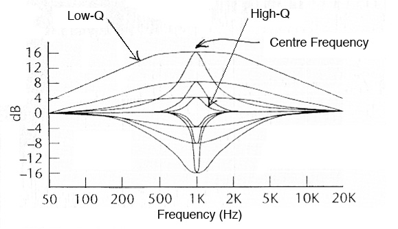
 Parametric equalizer frequency response for various values of Q
|  A useful subset of the parametric equalizer is the notch filter
which provides a very narrow attenuation of a specific frequency. The most
common use is for eliminating a 60 Hz hum (or 50 Hz in Europe). Similarly,
a
peak filter offers a single band similar to the parametric model.
Index
A useful subset of the parametric equalizer is the notch filter
which provides a very narrow attenuation of a specific frequency. The most
common use is for eliminating a 60 Hz hum (or 50 Hz in Europe). Similarly,
a
peak filter offers a single band similar to the parametric model.
Index
B. Interface representations of filters and equalizers.
Low-pass, high-pass and bandpass filters. These include a range of
graphic controls with virtual knobs and sliders, and a visual frequency
response diagram – which is useful, but don't take the shapes too
literally. Some allow the processing shapes to be stored for later use, and
most have some kind of bypass function to allow the effect to be turned off
and on, which is very useful for comparisons to the original, or in the
case
of multiple functions being used at the same time, to check the effect of
each one separately and as a set. Although this is a limited set that
compares 3 and 4 plug-ins, you should be able to find similar features in
other ones that you have available.
Many plug-ins offer several filter/EQ functions that are combined
in
one interface, but despite it being in software, the companies don't bother
to change the parameter names on the graphics, so you really need to know
your parameters to use them efficiently.
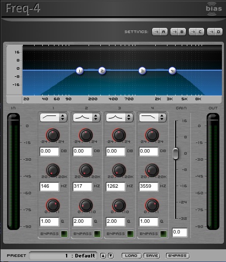
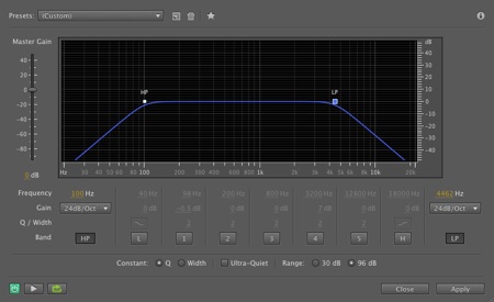
This simple 4-band plug-in has the typical high-pass and low-pass
curves as selected on bands 1 & 4. It allows you to sweep the white ball for each cut-off with a fixed roll-off.
The middle knob shows the cut-off frequency and allows control via the knob as a slider.
If the result is weak, the vertical slider at right allows for gain control. Bypass switches at the bottom.
| 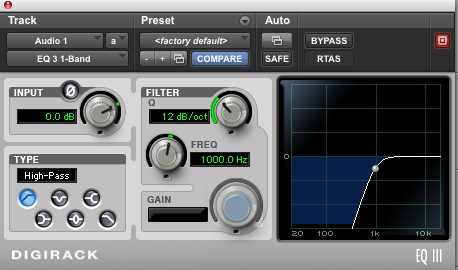
These are the standard ProTools single-band filters.
Note the icons for all the modes at the lower left.
On the right what is actually the roll-off is incorrectly called Q
and offers a choice from 6-24 dB/octave or more.
The cut-off frequency can be swept with the knob as a slider or by
dragging the white dot.
|
(click to enlarge)
This is the standard parametric processor in Audition which
includes
all of the standard processes, including high-pass (HP) and low-pass (LP)
at
the far left and right respectively.
A choice of cut-offs is offered, plus gain control at the left.
Because this is a digital filter, the roll-off can be chosen from 6 dB/oct
up to 48 dB/oct. However, note that all frequency changes in real time,
such
as the cut-offs, will result in clicks as they are moved.
|
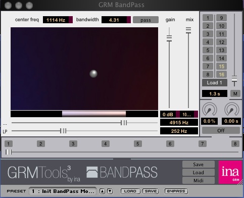
This is the standard bandpass model in GRM Tools, which comes in
both a mono and stereo version. Once you know how it works, the stereo
version is excellent for treating left and right channels independently
which will likely provide an interesting spatial spread to the timbre.
The x-axis is centre frequency and the y-axis is bandwidth, with
numerical values at the top, so both low-pass and high-pass functions are
neatly combined in a single gesture within the mouse paradigm. The actual
values in Hz for the two cut-offs are indicated in small windows to the
right of the individual manual controls for them. The other functions are
standard for all GRM functions and can be consulted in the documentation.
|
High and low shelf filters. These are the filters used to boost or
attenuate all low or high frequencies past a certain point.
The top diagram shows the low and high shelf filters (left and
right) attenuated, and the bottom diagram shows them boosted (probably
inadvisable), both in bands 1 and 4. The top two knobs control gain and cut
-off frequency respectively. Note the shelving pattern beyond those points
and compare it to the high-pass and low-pass filters above.
The top diagram shows the standard ProTools single-band filter in
low shelf mode with attenuation, and the bottom diagram shows the high
shelf
with positive gain.
Note the stirrup-shaped icons for these. The top slider knob
controls the steepness of the curve (called the Q); the cut-off frequency
and gain are controlled with the other two slider knobs.
(click to enlarge)
This diagram shows Audition’s standard parametric processor in
low
and high shelf mode together (marked L and H, not to be confused with HP
and
LP which are nearby).
The lows are being attenuated and highs boosted. This example uses
the “gentle slope” switch (above the L and H).
(click to enlarge)
This diagram shows Audition’s standard parametric processor in
low
and high shelf mode together (marked L and H, not to be confused with HP
and
LP which are nearby).
The lows are being attenuated and highs boosted. This example uses
the “steep slope” switch (above the L and H).
Peak and notch filters. These are subsets of the general parametric
model, offering one or two controllable bands.
The top diagram shows two bands (left and right) with a boost and
attenuation respectively, with a low Q, i.e. broad bandwidth. The bottom
diagram shows them with a high Q, i.e. narrow bandwidth, corresponding to
what otherwise might be called peak and notch modes. All three knobs are in
use to control (top to bottom) gain, centre frequency, and Q.
The top diagram shows the standard ProTools 1-band filter in peak
mode with a boost (that could be changed to attenuation with negative gain)
and choice of Q, in this case 1 which is quite broad.
The bottom diagram shows the specialized narrow-band notch filter
where the gain is maximized negatively, the Q value determines the
bandwidth, and the FREQ slider knob controls the centre frequency. Note the
different icons for each of these.
(click to enlarge)
This diagram shows Audition’s standard parametric processor used
with two bands simultaneously (marked 2 and 4). The lows are being boosted
in the first band and the highs attenuated in the second, but with a low Q
of 2, i.e. a broad bandwidth. Note that each band can be turned off and on.
(click to enlarge)
This diagram shows Audition’s standard parametric processor used
with two bands simultaneously (marked 2 and 4). The lows are being boosted
in the first band and the highs attenuated in the second, but with a high Q
of 10 (the max), i.e. a narrow bandwidth. Note that each band can be turned
off and on.
Full Parametric Equalizers. The Audition examples shown above were
all taken from its full parametric plug-in, so any of the various processes
could be added together. With ProTools, the 7-band parametric could look
intimidating, as shown next, despite being colour-coded, so again, it's
best
to learn each format thoroughly before using it.
Third-octave Equalizers. Unlike the interfaces for analog filters
and parametric equalizers, the interface paradigm for the third-octave
equalizer has not changed significantly in its migration into the digital
domain. Each band of filters is represented by a vertical line where the
vertical dimension represents gain above or below a zero point (i.e. where
no gain is applied). The bands themselves are identified by the centre
frequency based on the international standard of 1 kHz and its octaves and
sub-octaves. For a third-octave equalizer, there will be two additional
bands between each of those octaves.
Traditional analog 27-band graphic equalizer
Within a “mouse paradigm” where only one value can be adjusted
at a time, a serious problem arises for this kind of processor – how to
control its many variables efficiently. With the analog version, some skill
in using both sets of fingers to control multiple bands simultaneously
provided a certain kind of performability for dynamic changes. However, the
implied norm for its use was for a fixed setting: once the controls were
put
in place, they stayed there. The same applies to most plug-ins, but steps
can be taken for dynamic changes as discussed below.
We have already noted a significant extension to the “mouse
paradigm” with GRM Tools’ Bandpass model where two variables in the x-y
plane can be controlled by a the mouse on a small screen. However, unless
you have an extremely steady hand to move a mouse smoothly, dynamic changes
can sound jerky. GRM Tools solved this problem with the ability to
interpolate between presets with a ramp whose speed can be specified in a
small box below the presets (and stored with the preset). For filters and
equalizers, among others, these smooth ramps (which can be continuously
changed over time with multiple presets) offer an improvement over the
analog version in terms of performability.
Third-octave equalizer in Audition (click to enlarge)
The GRM Graphic Equalizer follows the standard paradigm with a few
differences. The EQ curve can be “drawn” by running the mouse over the
surface – but not too quickly – to trace a general curve. Then, each
band can be modified by dragging the gain of an individual band up or down
(with the corresponding centre frequency and gain indicated at the top).
Any
configuration can be stored as a preset. However, note that there is no
zero
line, and in fact the gain could be lowered to zero, unlike an analog
equalizer.
Rather unusually for GRM, the default group of presets are not
particularly useful, some being quite flat. An unusual configuration for
any
equalizer is to have alternate bands up and down, or every third one up –
the octave configuration. Given the 1/3 oct bandwidth, a spectral pitch
will
be heard even with noisy sounds, since any of these configurations
resembles
resonances in an air space. Musically, a third of an octave is a major
third, and every second band is an minor sixth apart, so some kinds of
tonal
sounding “chords” can be created.
Tip: The GRM Equalizer default presets have some of these
alternating band combinations, but since the lower gains go to zero, they
do
not cross-fade very smoothly, as the loudness drops in between presets.
Raising the low gains to a higher value will correct this issue.
Index
Circuits for using processors
C. Circuits for using processors. In the analog studio where
everything had to be patched (i.e. connected) together, creating a circuit
or signal path was absolutely fundamental as well as very flexible and open
-ended. Today, most signal paths are hidden or assumed, and at least one,
the parallel circuit is much more difficult to create and use. Before we
embark below on practical studio experiments, it would be useful to know
about some of these types of circuits, where your challenge will be how to
create them with your own equipment and software.
1. A direct recording refers to whatever route a signal takes from
the microphone to a sound file, where "mixer" might refer to a simple level
control. If you are importing a soundfile, then this step is not necessary.
2. A single transformation, or the "insert" version 2a, puts some
kind of processor in between the source and its subsequent saved output. In
the analog studio there was a subtle distinction about whether the
transformation happened before it arrived at the mixer or after. In digital
processing, the standard plug-in as illustrated above, is the equivalent to
this form of single transformation, and is usually provided on every track.
3. Likewise, if the software allows multiple plug-ins, the
assumption is that they are in a series configuration, that is, the output
of the first goes into the second, and so on. When using such multiples, it
is good to keep in mind that each process must be compatible with the
previous one. If the first is a filter that removes low frequencies, for
instance, they can’t be part of the processing in the second process.
4. The parallel circuit, in the analog tradition, relied on being
able to split the signal into exact copies, that is, multiple versions,
with
no loss of strength. This was accomplished with a special patch bay wiring
called a bridge or “multi” with several connections joined together
electrically to avoid signal loss. With one input, all the other
connections
could be outputs, and the multi could be patched to another for even more
outputs. These were then routed to independent processors and back into the
mixer to be combined. The beauty and simplicity of this setup was that all
signals were heard and processed in real time, and could be mixed in stereo
formats at will.
Today, auxiliary circuits can be used on a DAW or mixer for a real
-time version of the parallel circuit, but they are more complicated to set
up for beginners. Both a real-time and non-realtime version will be
described in the studio demo’s below as a kind of submix. All auxiliary
circuit, whether analog or digital, allow the signal to be sent to the
processing unit either independently of the playback level of the original
(called pre, meaning before the playback level), or at a level that depends
on the playback level (called post, meaning after the playback level and
therefore dependent on it).
5. A feedback circuit is one where the signal is fed back and mixed
with the original, but only where there’s enough of a delay involved that
it doesn’t immediately go into distortion, as indicated in the second
example above where the recording machine playback or a digital delay is
used. It can also be called recirculation because a loop has been set up.
The other requirement is a sensitive control over the feedback levels,
which
can increase the signal exponentially; that is, small changes become large
ones. Most of the examples of this approach will be described in the
modules
on Time Delays. However, feedback with filters at modest levels can make
them sound more like resonators.
Index
Introduction to Digital Filters using Waveguides
D. Introduction to Digital Filters using Waveguides. The topic of
digital filters from an engineering perspective is very complex, involving
differential equations in their design, and not all of them will be related
to sound design. However, it is still useful to consider some simple
examples of what are called 1st and 2nd order filters that can be modelled
using a short delay line also known as a waveguide. Basically, the
waveguide
is a memory array of n samples that are continuously stored and replaced
once full. Therefore the contents of the waveguide reflect the most recent
values of the waveform.
With these filter algorithms, only the previous sample, referred to
as x(n-1), or the second previous sample, x(n-2), are used, so the delay
line is very short, and in fact can be implemented with one or two
variables
that temporarily store these previous values.
The samples themselves are usually multiplied by a gain
coefficient,
often labelled g, and are combined with the direct signal which goes from
the input, x(n), to the output y(n) in these diagrams. The 1st order
examples are called that because they use only the previous sample, whereas
the 2nd order use the 2nd previous sample in the calculation.
Introducing the concepts of delay lines and waveguides here will
prepare the way for their use in longer lines for our presentation of
phasing (with short delays) and echo and reverb models (with long delays)
in
later modules.
These diagrams show four basic filters in terms of their frequency
response, equations and delay line circuits, from top to bottom. Here you
will see that the two 1st order models describe the familiar low-pass and
high-pass filters. The left-hand graphic circuit model shows that the input
signal at left goes into a delay line D, gets scaled by .5 and is combined
(the + sign) with the direct signal which is also multiplied by .5 to form
the output signal at the right.
This is a formal way of saying we are averaging the current sample
with the previous sample, since averaging involves adding two numbers
together and dividing by two. However, in the frequency domain, we have
learned that frequency is the rate of change of phase, with higher
frequencies showing a more rapid change of phase. When we average out those
rapid peaks, we are essentially filtering them out, hence the low-pass
effect.
Also note that the delay for the low-pass filter, D, is 1 sample
(i.e. first order), and for the band-reject filter D = 2, the second
previous sample, but otherwise the circuit is the same. Although simple, it
turns out that these filters are not very useful because the slope of their
roll-off is very gentle. Note also that the “zero” of the filter moves
from the half sampling rate (Fs) for the first-order filter, to half that
with the second-order filter (hence the term band reject).
For the two filters at the right, a similar process occurs, but
instead of averaging the adjacent samples, we subtract them from each
other.
Since low frequencies move slowly in terms of phase, adjacent samples will
show little difference in value, and therefore when samples are subtracted,
a small value will result. As noted, the 1st order version is a high-pass
filter, and the second order is a very simple bandpass filter. Note the
location of the zeroes in these filters, as well as their “poles” where
the output amplitude is highest. Higher orders in filter design using more
scaled previous samples would be needed to improve the roll-off.
Finally, we should note that these filters are called FIR filters,
Finite Impulse Response, because they settle to zero quickly, lacking any
feedback in the circuit that would prolong them.
However, when we model the resonances on a string (as in the first
Vibration module), there is feedback because of the waves are reflected at
both ends. Therefore, in the simple Karplus-Strong model of the string, as
shown below, there is an averaging function shown as a delay of one sample
(engineers refer to the length of the delay line with a z with an exponent
of -p where p is the length of the waveguide) in order to average the
value.
This acts as the simple low-pass filter shown above. Because of the
recirculation of the values in the waveguide, even the simplest low-pass
averaging filter will be effective because the filtering process happens
again and again.
The K-S model feeds its values back into the delay line (whose
length corresponds to that of the string), consistent with the standing
wave
phenomenon that is created in a real string. However, what we are
“processing” with a string is the initial energy applied to it, namely
the pluck, which is modelled by filling up the waveguide with random
numbers, but once filled, adding no more, similar to a single pluck. Note
the aural realism of the result including the decay of the sound
lengthening
with the length of the string/waveguide.
Karplus-Strong delay line resonator
Four plucks of the string model, with the waveguide length doubled
each time and the resulting spectrogram
To complete this brief survey of digital filters, we have two more
diagrams, the one at left showing an Infinite Impulse Response filter (IIR)
which incorporates both the feed forward function that we saw above, that
is, adding two previous input samples, x(n-1) and x(n-2), to the direct
signal, as well as a feedback function that recirculates two of the
previous
output samples, y(n-1) and y(n-2). Note the gain values called coefficients
are the various a, b values. This feedback function creates the
“ringing” behaviour of theoretically infinite repetitions, similar to
the various forms of audio feedback we will encounter later. Careful
control
over the feedback level will affect how long it lasts.
The right hand diagram shows an all-pass filter which means that
all
frequencies are passed equally, that is, with the same gain, but there are
predictable phase shifts in certain frequencies.
Keep in mind that the two most salient points in this topic are
that:
manipulation of the time domain in terms of delay samples
affects the frequency domain (a characteristic of microsound)
filters can exhibit resonating behaviour when feedback is
involved
Try this review quiz
Q. Try this review quiz to test your comprehension of the above
material (not including Digital Filters), and perhaps to clarify some
distinctions you may have missed. Note that a few of the questions may have
"best" and "second best" answers to explain these distinctions.
Index
Studio Demo's and Personal Projects
E. Studio Demo's and Personal Projects. With some exceptions, we
will not be referencing specific equipment in these demo’s, but for you
to
replicate them (definitely a good idea), you will need to find equivalent
solutions with whatever software you have available. However, we are
recommending that you use both a waveform editor with whatever plug-ins it
is equipped with for processing, and a DAW (digital audio workstation) for
assembling and mixing your files. Some waveform editors, such as Audition,
include a small mixing module where multiple tracks can be combined. This
can be useful for test mixes and submixes, i.e. where you combine multiple
versions of your sounds into a mix that can be bounced into a cumulative
file.
a) Demo's using filters and equalizers.
b) Personal studio experiment No. 1.
c) Parallel circuit models demo's.
d) Personal studio experiment No. 2.
a. Using filters and equalizers. In starting a project or
experiment, the so-called raw recording you intend to use will likely need
to be edited and cleaned up. Some users will prefer to keep the original
recording intact, for future reference, whereas others might already delete
any extraneous sounds and adjust levels (particularly when the record level
is low) with the editor.
After you’ve made those choices, the next stage of clean-up might
be to use a filter to get rid of unwanted low frequencies, for instance.
Even if you end up using only a subset of the entire source soundfile (see
the personal experiments below), it is a good idea to have all of it
cleaned
up in this manner first, so you won’t have to do it again if you go back
to the original (and forget how you cleaned it up).
1. Using a high-pass filter.
Original scything recording with wind noise
Source: WSP Canada 32 take 10
Waveform prior to filtering
Recording processed with a high-pass filter
Waveform after filtering
|
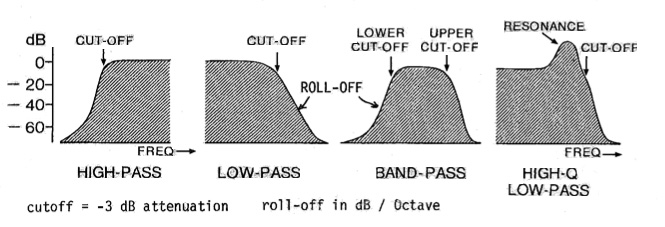 At the left we have the high-pass and low-pass filters. They have
two variables, the cut-off frequency which is where the signal is
attenuated
by 3 dB (that is, where the attenuation is regarded as significant), and
the
roll-off which is the slope of the filter’s response beyond the cut-off.
In other words, the term “cut” is not an accurate description of the
filter’s action as it implies removing something (true), but in a clean
and precise manner (not possible). All filters, whether analog of digital,
cannot eliminate, for instance, all frequencies below exactly 100 Hz, which
would require a rectangular response.
Instead, all frequencies below the cut-off of a high-pass filter
are
gradually attenuated according to the slope of the roll-off. Because it can
be thought of as a slope, the units are decibels per octave, in other
words,
it specifies how much attenuation there is with each octave. It might help
to think of the slope of a highway, the grade, expressed as a percentage.
With a roll-off of 12 dB/oct and a cutoff of 100 Hz (which is attenuated 3
dB by definition), the attenuation at 50 Hz (an octave lower) would be 3 +
12 = 15 dB.
The important distinction is that the larger the roll-off value,
the
more precisely it distinguishes between the desired frequencies that remain
(i.e. are passed) and those which are attenuated. Today, digital filters
typically have slopes of 16, 24 or more (e.g. 48 dB/octave) which is more
than enough to isolate a frequency band cleanly. The limiting factor to
having an extremely steep slope is that it adds phase distortion to the
sound, hence the impossibility of having a rectangular cut.
In analog filters, the roll-off is fixed by the circuitry and
cannot
be changed. In digital filters, the roll-off is calculated as variables in
an equation. Therefore, you can only select a desired roll-off and switch
to
it, as opposed to the cut-off frequency which can be swept up or down
continuously at will, an interactive ability that is aurally very effective
for hearing the changes in the spectrum.
Also, this type of sweep often produces an aurally interesting way
of introducing a sound into a mix, starting with a high cutoff in a high
-pass filter and lowering it gradually, or vice versa with a low-pass
filter, an alternative to the conventional fade-in. A good digital filter
will not have clicks when the cut-off is swept, so be careful with any that
produce this kind of artifact.
The bandpass filter, shown above, is the combination (quite
literally) of these two filters, the high-pass and low-pass. It is
controlled by two cut-offs, low and high, with the distance between them
referred to as the passband. Because there are two variables in a bandpass
filter (plus the roll-off), a digital application will have to decide if
there are two separate controls, and if so, which ones.
One choice that works well is centre frequency and bandwidth (to
borrow terms from the Equalizer). If the control surface is a two
-dimensional window with an X-Y axis, then this double choice could work
well for a mouse moving around the space (for instance, as found in the GRM
Tools approach, as shown below).
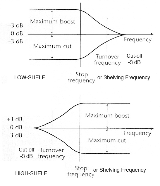
As briefly mentioned above, the shelf filter is a hybrid between a
low-pass (or high-pass) filter and an equalizer. The difference is the lack
of a continuous roll-off. All frequencies below the cut-off or turnover
frequency in a low shelf filter are either boosted or attenuated (that is,
+
or - gain in decibels). Once the gain is decided, that is the gain for all
frequencies below what is called the stop frequency or shelving frequency.
Something similar happens with a high shelf, except that the gain
is
for frequencies above the cut-off or turnover frequency. In practice, the
shelf filter seems cruder than the bandpass, particularly when it is
attenuating. In terms of low frequencies, the high-pass filter will
progressively eliminate them, whereas a low shelf filter will merely lower
them in intensity. Presumably the difference is whether removing or simply
lowering those frequencies is the desired goal. Use of the shelf filter to
boost all highs or lows should be done carefully, if at all.
At the left we have the high-pass and low-pass filters. They have
two variables, the cut-off frequency which is where the signal is
attenuated
by 3 dB (that is, where the attenuation is regarded as significant), and
the
roll-off which is the slope of the filter’s response beyond the cut-off.
In other words, the term “cut” is not an accurate description of the
filter’s action as it implies removing something (true), but in a clean
and precise manner (not possible). All filters, whether analog of digital,
cannot eliminate, for instance, all frequencies below exactly 100 Hz, which
would require a rectangular response.
Instead, all frequencies below the cut-off of a high-pass filter
are
gradually attenuated according to the slope of the roll-off. Because it can
be thought of as a slope, the units are decibels per octave, in other
words,
it specifies how much attenuation there is with each octave. It might help
to think of the slope of a highway, the grade, expressed as a percentage.
With a roll-off of 12 dB/oct and a cutoff of 100 Hz (which is attenuated 3
dB by definition), the attenuation at 50 Hz (an octave lower) would be 3 +
12 = 15 dB.
The important distinction is that the larger the roll-off value,
the
more precisely it distinguishes between the desired frequencies that remain
(i.e. are passed) and those which are attenuated. Today, digital filters
typically have slopes of 16, 24 or more (e.g. 48 dB/octave) which is more
than enough to isolate a frequency band cleanly. The limiting factor to
having an extremely steep slope is that it adds phase distortion to the
sound, hence the impossibility of having a rectangular cut.
In analog filters, the roll-off is fixed by the circuitry and
cannot
be changed. In digital filters, the roll-off is calculated as variables in
an equation. Therefore, you can only select a desired roll-off and switch
to
it, as opposed to the cut-off frequency which can be swept up or down
continuously at will, an interactive ability that is aurally very effective
for hearing the changes in the spectrum.
Also, this type of sweep often produces an aurally interesting way
of introducing a sound into a mix, starting with a high cutoff in a high
-pass filter and lowering it gradually, or vice versa with a low-pass
filter, an alternative to the conventional fade-in. A good digital filter
will not have clicks when the cut-off is swept, so be careful with any that
produce this kind of artifact.
The bandpass filter, shown above, is the combination (quite
literally) of these two filters, the high-pass and low-pass. It is
controlled by two cut-offs, low and high, with the distance between them
referred to as the passband. Because there are two variables in a bandpass
filter (plus the roll-off), a digital application will have to decide if
there are two separate controls, and if so, which ones.
One choice that works well is centre frequency and bandwidth (to
borrow terms from the Equalizer). If the control surface is a two
-dimensional window with an X-Y axis, then this double choice could work
well for a mouse moving around the space (for instance, as found in the GRM
Tools approach, as shown below).
As briefly mentioned above, the shelf filter is a hybrid between a
low-pass (or high-pass) filter and an equalizer. The difference is the lack
of a continuous roll-off. All frequencies below the cut-off or turnover
frequency in a low shelf filter are either boosted or attenuated (that is,
+
or - gain in decibels). Once the gain is decided, that is the gain for all
frequencies below what is called the stop frequency or shelving frequency.
Something similar happens with a high shelf, except that the gain
is
for frequencies above the cut-off or turnover frequency. In practice, the
shelf filter seems cruder than the bandpass, particularly when it is
attenuating. In terms of low frequencies, the high-pass filter will
progressively eliminate them, whereas a low shelf filter will merely lower
them in intensity. Presumably the difference is whether removing or simply
lowering those frequencies is the desired goal. Use of the shelf filter to
boost all highs or lows should be done carefully, if at all.
 Equalizers (used to EQ a sound) come in many variations, the main
one being how many bands are available, the more the better, in general. It
is useful to think of an equalizer as a set of filters, where each band has
a fixed bandwidth, usually defined in octaves and fractions thereof.
However, unlike the filters we've considered, gain can be applied to boost
or attenuate each band.
A third-octave bandwidth, meaning 3 separate bands per octave (with
a total of between 24 and 30 bands to control) is a standard. When we study
the ear’s resolving power for frequencies in a spectrum, called the
critical bandwidth (that will be deal with in the second Vibration module),
we will find that it is a little less than a quarter of an octave, so the
1/3 octave equalizer comes close to controlling exactly the range of
frequencies that we can hear separately in a spectrum.
The diagram below, if taken literally, would not be a very good
equalizer as it only has 7 bands to cover a 9-octave range of frequencies,
even though they are distributed on a logarithmic frequency scale. So, each
band covers over an octave, which might make it easy to use in a car audio
system, but it is ill-suited for audio design work. The saving grace of the
diagram is that it is easier to see what is going on than, say, with a 24
-band equalizer.
The controls on an equalizer, for each band, are the choice of
centre frequency and the gain, plus or minus, which is continuously
variable
up to or down to a maximum, here shown as +/- 12, but more typically +/- 15
or 20. In general it is the “curved” shape of this set of gains that is
most effective, rather than the maximum gain. In fact, so much gain can be
cumulatively applied with an equalizer that the sound will distort and/or
be
unpleasant to our ears, particularly if the boost is in the 1-4 kHz range
where the ear is most sensitive.
Equalizers (used to EQ a sound) come in many variations, the main
one being how many bands are available, the more the better, in general. It
is useful to think of an equalizer as a set of filters, where each band has
a fixed bandwidth, usually defined in octaves and fractions thereof.
However, unlike the filters we've considered, gain can be applied to boost
or attenuate each band.
A third-octave bandwidth, meaning 3 separate bands per octave (with
a total of between 24 and 30 bands to control) is a standard. When we study
the ear’s resolving power for frequencies in a spectrum, called the
critical bandwidth (that will be deal with in the second Vibration module),
we will find that it is a little less than a quarter of an octave, so the
1/3 octave equalizer comes close to controlling exactly the range of
frequencies that we can hear separately in a spectrum.
The diagram below, if taken literally, would not be a very good
equalizer as it only has 7 bands to cover a 9-octave range of frequencies,
even though they are distributed on a logarithmic frequency scale. So, each
band covers over an octave, which might make it easy to use in a car audio
system, but it is ill-suited for audio design work. The saving grace of the
diagram is that it is easier to see what is going on than, say, with a 24
-band equalizer.
The controls on an equalizer, for each band, are the choice of
centre frequency and the gain, plus or minus, which is continuously
variable
up to or down to a maximum, here shown as +/- 12, but more typically +/- 15
or 20. In general it is the “curved” shape of this set of gains that is
most effective, rather than the maximum gain. In fact, so much gain can be
cumulatively applied with an equalizer that the sound will distort and/or
be
unpleasant to our ears, particularly if the boost is in the 1-4 kHz range
where the ear is most sensitive.
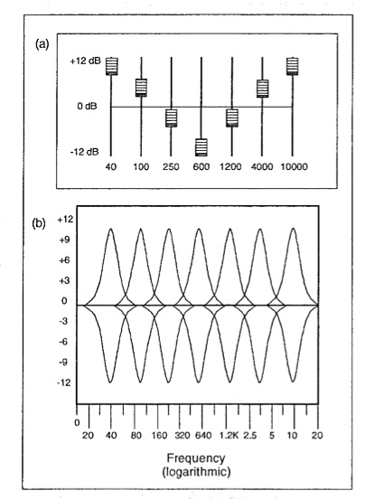 Multi-band equalizer (a) and its frequency response pattern (b)
Parametric Equalizer. A parametric equalizer makes all of its
variables controllable, namely:
Centre Frequency (CF) in Hz or kHz
Gain in + or - dB
Bandwidth as the ratio Q where Q = Centre Frequency / Bandwidth
If the last controllable parameter (Q) were actually bandwidth, it
would be difficult to use because of the logarithmic nature of frequency.
For instance, from 100 to 200 Hz is an octave, and the bandwidth is 100 Hz;
the octave from 1 kHz to 2 kHz represents a bandwidth of 1000 Hz. So, if we
kept the bandwidth constant at 100 Hz, and swept the centre frequency from
100 Hz to 1 kHz, we’d go from a very large bandwidth to a very narrow one
perceptually, with resulting inconsistency in how the result would sound.
Admittedly we could keep it constant as a ratio with an interval of, say,
1/3 octave, but that isn’t very easy to specify in general.
Therefore, by creating the unitless ratio of Q, being the ratio
between the centre frequency and the bandwidth, we keep the actual
bandwidth
comparable at all centre frequencies. The usual range of Q is from 1 to 10,
or higher in digital versions, which can also be thought of as a range of
bandwidths from being equal to the centre frequency to being 1/10 of it for
Q = 10.
Narrow bandwidths, with a Q above 5 or 6, may be narrow enough
that,
when applied to broadband sounds, a spectral pitch will emerge, somewhat
similar to a vocal formant which is a narrow resonance region that helps to
identify a vowel. The diagram below shows the range of Q from low (i.e.
broad bandwidth) to high (i.e. very narrow bandwidth) at different gain
levels for clarity.
In general, the Q factor should be judged carefully by ear to being
just enough to give the sound more focus and presence, but not so much as
to
be annoyingly intrusive (since the auditory system is very focused on
picking up such resonance regions). This type of boost in the 2-3 kHz
region
will give speech added presence and clarity, as demonstrated later.
Multi-band equalizer (a) and its frequency response pattern (b)
Parametric Equalizer. A parametric equalizer makes all of its
variables controllable, namely:
Centre Frequency (CF) in Hz or kHz
Gain in + or - dB
Bandwidth as the ratio Q where Q = Centre Frequency / Bandwidth
If the last controllable parameter (Q) were actually bandwidth, it
would be difficult to use because of the logarithmic nature of frequency.
For instance, from 100 to 200 Hz is an octave, and the bandwidth is 100 Hz;
the octave from 1 kHz to 2 kHz represents a bandwidth of 1000 Hz. So, if we
kept the bandwidth constant at 100 Hz, and swept the centre frequency from
100 Hz to 1 kHz, we’d go from a very large bandwidth to a very narrow one
perceptually, with resulting inconsistency in how the result would sound.
Admittedly we could keep it constant as a ratio with an interval of, say,
1/3 octave, but that isn’t very easy to specify in general.
Therefore, by creating the unitless ratio of Q, being the ratio
between the centre frequency and the bandwidth, we keep the actual
bandwidth
comparable at all centre frequencies. The usual range of Q is from 1 to 10,
or higher in digital versions, which can also be thought of as a range of
bandwidths from being equal to the centre frequency to being 1/10 of it for
Q = 10.
Narrow bandwidths, with a Q above 5 or 6, may be narrow enough
that,
when applied to broadband sounds, a spectral pitch will emerge, somewhat
similar to a vocal formant which is a narrow resonance region that helps to
identify a vowel. The diagram below shows the range of Q from low (i.e.
broad bandwidth) to high (i.e. very narrow bandwidth) at different gain
levels for clarity.
In general, the Q factor should be judged carefully by ear to being
just enough to give the sound more focus and presence, but not so much as
to
be annoyingly intrusive (since the auditory system is very focused on
picking up such resonance regions). This type of boost in the 2-3 kHz
region
will give speech added presence and clarity, as demonstrated later.